
Chapter 3. Develop queries using Multidimensional Expressions (MDX) and Data Analysis Expressions (DAX)
SQL Server Analysis Services (SSAS) multidimensional and tabular models rely on separate expression languages for both modeling and querying purposes. You use the Multidimensional Expressions (MDX) language to incorporate business logic into a cube for reusability as calculations and to return query results from a cube. Cube queries can be ad hoc, embedded into a reporting application, or generated automatically by client tools such as Excel. Likewise, you use the Data Analysis Expressions (DAX) language to enhance a tabular model not only by adding business logic, but also to perform data transformation tasks such as concatenating or splitting strings, among other tasks. In addition, you use DAX to query a tabular model in ad hoc or reporting tools. Client tools, such as Power BI Desktop and Power View in SQL Server Reporting Services (SSRS) and in Excel, can generate DAX. The 70-768 exam tests your knowledge of both MDX and DAX to ensure you have the skills necessary to build and query multidimensional or tabular models effectively.
Skills in this chapter:
![]() Implement custom MDX solutions
Implement custom MDX solutions
![]() Create formulas by using the DAX language
Create formulas by using the DAX language
Skill 3.1: Create basic MDX queries
Before you start adding MDX calculations into a multidimensional model, you may find it easier to first test the calculations by executing an MDX query in SQL Server Management Studio (SSMS). Furthermore, even when users rely on tools that automatically generate MDX, you should have an understanding of how to write MDX queries so that you have a foundation for the skills necessary to troubleshoot performance issues, as described in Chapter 4, “Configure and maintain SQL Server Analysis Services (SSAS).”
Implement basic MDX structures and functions, including tuples, sets, and TopCount
Before you start writing MDX queries, you should be familiar with the terms used to describe objects in the multidimensional database. Because many of these objects are visible in the metadata pane in the MDX query window, it’s helpful to review the contents of the metadata pane to familiarize yourself with accessible objects and available MDX functions.
Note Sample multidimensional database for this chapter
This chapter uses the database created in Chapter 1, “Design a multidimensional business intelligence (BI) model,” to illustrate MDX concepts and queries. If you have not created this database, you can restore the ABF file included with this chapter’s code sample files. To do this, copy the 70-768-Ch1.ABF file from the location in which you stored the code sample files for this book to the Backup folder for your SQL Server instance, such as C:Program FilesMicrosoft SQL ServerMSAS13.MSSQLSERVEROLAPBackup. Then open SQL Server Management Studio (SSMS), select Analysis Services in the Server Type drop-down list, provide the server name, and click Connect. In Object Explorer, right-click the Databases folder, and click Restore Database. In the Restore Database dialog box, click Browse, expand the Backup path folder, and select the 70-768-Ch1.ABF file, and click OK. In the Restore Database text box, type 70-768-Ch1, and click OK.
Basic MDX objects
Let’s start by reviewing the structure of the 70-768-Ch1 database by following these steps:
1. If necessary, open SSMS, select Analysis Services in the Server Type drop-down list, provide the server name, and click Connect.
2. In the toolbar, click the Analysis Services MDX Query button and then, in the Connect To Analysis Services dialog box, click Connect.
3. If it is not already set as the current database, select 70-768-Ch1 in the Available Databases drop-down list in the toolbar.
4. In the Cube drop-down list in the metadata pane to the left of the query window, select Wide World Importers DW.
5. In the metadata pane, expand the Measures folder and the Sale folder. Then expand the Date dimension folder, the Date.Calendar attribute folder, and the Calendar Year level folder. With these folders expanded, as shown in Figure 3-1, you can see the following structures:
![]() Measure group Collection of measures.
Measure group Collection of measures.
![]() Measure Numeric value, typically aggregated.
Measure Numeric value, typically aggregated.
![]() Calculated measure Calculated value, typically aggregated.
Calculated measure Calculated value, typically aggregated.
![]() Dimension Container for a set of related attributes used to analyze numeric data.
Dimension Container for a set of related attributes used to analyze numeric data.
![]() Attribute hierarchy Typically a two-level hierarchy containing an All member and distinct attribute values (members) from a dimension column.
Attribute hierarchy Typically a two-level hierarchy containing an All member and distinct attribute values (members) from a dimension column.
![]() Level Label for a collection of attributes in a user-defined hierarchy.
Level Label for a collection of attributes in a user-defined hierarchy.
![]() Member Individual item in an attribute.
Member Individual item in an attribute.
![]() User-defined hierarchy Collection of levels, typically structured as a natural hierarchy with levels having a one-to-many relationship between parent and child levels. An unnatural hierarchy has a many-to-many relationship between parent and child levels.
User-defined hierarchy Collection of levels, typically structured as a natural hierarchy with levels having a one-to-many relationship between parent and child levels. An unnatural hierarchy has a many-to-many relationship between parent and child levels.

MDX query structure
The basic structure of an MDX query looks similar to a Structured Query Language (SQL) query because it includes a SELECT clause and a FROM clause, but that’s the end of the similarity. For example, the simplest MDX that you can write for the Wide World Importers DW cube is shown in Listing 3-1, and the query result is shown in Figure 3-2. You must type the SELECT FROM portion of the query, and then either type the cube name or drag the cube name from the metadata pane and drop it after FROM. Although optional, it is considered best practice to terminate your query with a semi-colon as a security measure to prevent an MDX injection attack.
LISTING 3-1 Simplest MDX query
SELECT
FROM
[Wide World Importers DW];

Normally, the SELECT clause includes additional details to request SSAS to retrieve information for specific dimensions and measures, but Listing 3-1 omits these details. The FROM clause identifies the cube to query.
How does SSAS know what to return as the result in this example? Part of the answer is in the following concepts to always keep in mind whenever you write your own queries:
![]() Default member Each attribute hierarchy in each dimension in the cube has a DefaultMember property. If you do not explicitly define a default member, as described in Skill 3.2, “Implement custom MDX solutions,” SSAS implicitly considers the All member at the top level of an attribute hierarchy to be the default member.
Default member Each attribute hierarchy in each dimension in the cube has a DefaultMember property. If you do not explicitly define a default member, as described in Skill 3.2, “Implement custom MDX solutions,” SSAS implicitly considers the All member at the top level of an attribute hierarchy to be the default member.
![]() Default measure The cube has a DefaultMeasure property. Like default members, you can either explicitly define a value for this property, or understand how SSAS implicitly defines a default measure. To find the implicit default measure, you must review the cube’s measures on the Cube Structure page of the cube designer. Expand the first measure group’s folder and take note of the first measure in this folder because this is the implicit default member. It is important to note that you cannot determine the default measure by reviewing the sequence of measures in the metadata pane in the MDX query window in SSMS or in the Browser page of the cube designer in SQL Server Data Tools for Visual Studio Tools 2015 (SSDT).
Default measure The cube has a DefaultMeasure property. Like default members, you can either explicitly define a value for this property, or understand how SSAS implicitly defines a default measure. To find the implicit default measure, you must review the cube’s measures on the Cube Structure page of the cube designer. Expand the first measure group’s folder and take note of the first measure in this folder because this is the implicit default member. It is important to note that you cannot determine the default measure by reviewing the sequence of measures in the metadata pane in the MDX query window in SSMS or in the Browser page of the cube designer in SQL Server Data Tools for Visual Studio Tools 2015 (SSDT).
Based on this information, the result of 8,951.628 represents the aggregated value for Quantity for all members of all attribute hierarchies of all dimensions. You could derive the same result by listing each individual All member along with the Quantity member, but to do so would be a tedious process. Instead, you can take advantage of the assumptions that the SSAS engine makes about your query to create a more succinct query. At times, an MDX query for a cube can be much more compact than an equivalent SQL query for a relational database. For this example, you can translate the MDX query in Listing 3-1 to the SQL query shown in Listing 3-2.
LISTING 3-2 Equivalent SQL query
SELECT SUM(Quantity)
FROM
WideWorldImportersDW.Sales.Fact;
Because the default measure can change if new measures are added to the cube, you should explicitly request the measure (or measures) that you want to return in the query results, as shown in Listing 3-3. This time, the measure is named in the SELECT clause, but notice the clause includes ON COLUMNS after the measure name also. Figure 3-3 shows the same value that was returned in the original form of the query, but the results also include a column label for this value thereby removing any ambiguity about what the value represents.
LISTING 3-3 MDX query with single measure
SELECT
[Measures].[Quantity] ON COLUMNS
FROM
[Wide World Importers DW];

While a query with a single measure can be useful for some questions, many times you want to break down, or slice and dice, a measure by a single member or multiple members of a dimension. To add a single dimension member to the query, you extend the SELECT clause by adding a comma, specifying the member name, and appending ON ROWS, as shown in Listing 3-4. You can see the result of the query in Figure 3-4, which shows the member name as a label on rows, the measure name as a label on columns, and the value 1,101,101 displayed at the intersection of the measure and dimension member.
LISTING 3-4 MDX query with single measure and single dimension member
SELECT
[Measures].[Quantity] ON COLUMNS,
[Stock Item].[Color].[Black] ON ROWS
FROM
[Wide World Importers DW];

Note Axis naming and order options
When you reference columns and rows in an MDX query, you are referencing axes in the query. In the query, you can use replace ON COLUMNS with ON 0 and ON ROWS with ON 1. In addition, when you include both axes in a query, you can place the ON ROWS clause before the ON COLUMNS clause if you like. However, if you include only one axis in the query, you must include the columns axis. A query that includes only the ON ROWS clause is not valid.
A query can be more complex, of course. Before exploring query variations, you should be familiar with the general structure of an MDX query, which looks like this:
SELECT
<Set> ON COLUMNS,
<Set> ON ROWS
FROM
<Cube>
WHERE
<Tuple>;
Members and sets
Sets are an important concept in MDX. A set is a collection of members from the same dimension and hierarchy. The hierarchy can be an attribute hierarchy or a user-defined hierarchy. There are several different ways that you can reference a member that use legal syntax, but best practice is to use the member’s qualified name. The qualified name is an identifier for a member than uniquely identifies it within a cube. A member’s unique name includes both the dimension and hierarchy name as prefixes to the member, uses a period (.) as a delimiter between object names, and encloses each object name in brackets like this:
[Stock Item].[Color].[Black]
Another way to reference a dimension member is to use its key column value, also known as its unique name. Recall from Chapter 1 that each attribute has a KeyColumn and NameColumn property. Although it is easier to read a query that references members by using the NameColumn values, such as Stock Item].[Stock Item].[USB missile launcher (Green)], you should consider writing a query to use the KeyColumn values when the possibility exists that the NameColumn values can change, such as when the attribute is handled as a Type 1 slowly changing dimension as described in Chapter 1. In that case, the syntax for a dimension member’s unique name appends an ampersand (&) prior to the KeyColumn value like this:
[Stock Item].[Stock Item].&[1]
Note Unique names in metadata pane
When you hover your cursor over a member name in the metadata pane, you can see its key value. Furthermore, when you drag the member name from the metadata pane into the query window in SSMS, the member’s unique name is added to the query. If you prefer to use the qualified name, you must type the member’s qualified name into the query.
Table 3-1 shows examples of different types of sets. You always enclose a set in braces, unless the set consists of a single member or the set is returned by a function. Set functions are explained in more detail later in this section. Experiment with these set types by replacing the set on columns in the query shown in Listing 3-4 with the example shown in the table.

Important Mixing attributes from multiple hierarchies is invalid
You cannot combine attributes from separate hierarchies of the same dimension into a single set. As an example, you cannot create a set like this: {[Stock Item].[Color].[Black],[Stock Item].[Size].[L]}
When you explicitly define the members in a set by listing the members and enclosing them in braces, the order in which the members appear in the set is the order in which they appear when you add them to the query. When you use a set function like Members, the OrderBy property for the attribute determines the sort order of those members in the query results. You can override this behavior as explained later in this chapter when commonly used functions are introduced.
Measures can also be members of a set. From the perspective of creating MDX queries, measures belong to the Measures dimension, but do not belong to a hierarchy. Therefore, you can create a set of measures like this:
{[Measures].[Sales Amount Without Tax], [Measures].[Profit]}
In most cases, you can put a measure set on either axis of the query results. Listing 3-5 shows two queries containing the same sets, but each query has its sets on opposite axes. Notice that you can place the GO command between MDX queries to enable the execution of both statements at one time. Figure 3-5 shows the results of both queries.
LISTING 3-5 Comparing queries with sets on opposite axes
SELECT
{[Measures].[Sales Amount Without Tax], [Measures].[Profit]} ON COLUMNS,
{[Stock Item].[Color].[Black], [Stock Item].[Color].[Blue]} ON ROWS
FROM
[Wide World Importers DW];
GO
SELECT
{[Stock Item].[Color].[Black], [Stock Item].[Color].[Blue]} ON COLUMNS,
{[Measures].[Sales Amount Without Tax], [Measures].[Profit]} ON ROWS
FROM
[Wide World Importers DW];

The exception to this ability to place measures on either axis is the construction of a query for SSRS. In that case, not only must you place the measure set on the columns axis, but also it is the only type of set that you can place on the columns axis.
Tuples
Tuples are another important concept in MDX. A tuple is a collection of members from different dimensions and hierarchies that is enclosed in parentheses. Conceptually, a tuple is much like a coordinate to a specific cell in a cube. Consider the simple example shown in Figure 3-6, which depicts a cube that contains a Date dimension with a Month attribute hierarchy, a Territory dimension with a Territory attribute hierarchy, and a single measure, Sales Amount.

To retrieve a value from a specific cell in this simple cube, such as the Sales Amount for the North territory in the month of January as shown in Figure 3-7, you create a tuple that references every dimension and the one measure in the cube, like this:
([Territory].[Territory].[North], [Date].[Month].[January], [Measures].[Sales Amount])

Note Order of members in a tuple has no effect on result
The order of members in a tuple does not affect the result returned by a query. Thus, the following three tuples yield the same answer:
([Territory].[Territory].[North], [Date].[Month].[January],
[Measures].[Sales Amount])
([Date].[Month].[January], [Measures].[Sales Amount], [Territory].
[Territory].[North])
([Measures].[Sales Amount], [Territory].[Territory].[North], [Date].[Month].
[January])
You can create a tuple that omits one of the dimensions or the measure also. In that case, the tuple implicitly includes the default member or default measure to create a complete tuple behind the scenes. Therefore, the tuple ([Date].[Month].[January], [Measures].[Sales Amount]) is the equivalent of ([Territory].[Territory].[All Territories], [Date].[Date].[Month], [Measures].[Sales Amount]) as shown in Figure 3-8.

MDX query syntax does not allow you to place a tuple on an axis. Only sets are permissible on rows or columns. Instead, you place a tuple in the WHERE clause, which is not intuitive if you are accustomed to writing SQL queries. Whereas a SQL query relies on a WHERE clause to define a filter condition, the WHERE clause in an MDX query affects how the SSAS formula engine constructs the tuples that it retrieves from the cube to generate a query’s results.
For example, a simple query that requests a specific tuple from the Wide World Importers DW cube is shown in Listing 3-6 and the result in SSMS is shown in Figure 3-9. Notice there is no label on rows or columns, because the query does not include a specification on the rows or columns axis. Nonetheless, the value of $3,034,239.00 is the query result. This value reflects sales for all stock items that have the color of black for all dates, all cities associated with the Far West default member (defined in Chapter 1), all customers, and so on.
LISTING 3-6 MDX query with a tuple
SELECT
FROM
[Wide World Importers DW]
WHERE
([Measures].[Sales Amount Without Tax],
[Stock Item].[Color].[Black]);

Another way to request the same tuple in a query is shown in Listing 3-7. The result shown in Figure 3-10 now includes the labels for the row and column. The difference between the two queries is the structure of the query command and the presentation of the results.
LISTING 3-7 MDX query with single members on each axis to create a tuple
SELECT
[Measures].[Sales Amount Without Tax] ON COLUMNS,
[Stock Item].[Color].[Black] ON ROWS
FROM
[Wide World Importers DW];
Yet another way to define a tuple to retrieve for a query is to include some objects on the axis and other objects in the WHERE clause, as shown in Listing 3-8. The SSAS formula engine combines objects from rows, columns, and the WHERE clause to construct the tuple that it returns in the results, shown in Figure 3-11.
LISTING 3-8 MDX query with single members on each axis and in the WHERE clause to create a tuple
SELECT
[Measures].[Sales Amount Without Tax] ON COLUMNS,
[Stock Item].[Color].[Black] ON ROWS
FROM
[Wide World Importers DW]
WHERE
([Invoice Date].[Calendar Year].[CY2016]);

Tuple sets
To create a more complex query, you can create a tuple set and use it on a query axis. A tuple set is a set comprised of tuples in which a comma separates each tuple and braces enclose the entire set. Each tuple in the set must be consistent in the number of objects, the order of those objects, and the dimensions and hierarchies in which those objects belong. A valid tuple set looks like this:
{ ([Measures].[Sales Amount Without Tax], [Invoice Date].[Calendar Year].[CY2016]),
([Measures].[Sales Amount Without Tax], [Invoice Date].[Calendar Year].[CY2015]),
([Measures].[Sales Amount Without Tax], [Invoice Date].[Calendar Year].[CY2014]) }
By contrast, an invalid tuple set looks like this:
{ ([Measures].[Sales Amount Without Tax], [Invoice Date].[Calendar Year].[CY2016]),
([Invoice Date].[Calendar Year].[CY2015], [Measures].[Sales Amount Without Tax]),
([Measures].[Sales Amount Without Tax], [City].[Sales Territory].[Southwest]) }
Listing 3-9 provides an example of an MDX query in which tuple sets are placed on both axes. In Figure 3-12, you can see the relationship between the query elements, tuple construction, and the query results. The SSAS formula engine processes the query in multiple steps. In Steps 1 and 2, the engine retrieves members from the respective dimensions and hierarchies to construct the axes. In Step 3, the final tuples are constructed cell-by-cell and the engine determines how best to retrieve those values from the cube—in bulk or cell-by-cell as explained in greater detail in Chapter 4, “Configure and maintain SQL Server Analysis Services (SSAS).” Because the combination of rows and columns results in six cells, SSAS constructs six tuples. Each tuple includes the members shown in the column header and the row header for its cell in addition to the members in the WHERE clause. Thus, the WHERE clause is a subset of the tuple in each cell and results in the retrieval of data from a different location in the cube than the location used if the WHERE clause were omitted.
LISTING 3-9 MDX query with tuple sets
SELECT
{ ([Measures].[Sales Amount Without Tax], [Invoice Date].[Calendar Year].[CY2016]),
([Measures].[Sales Amount Without Tax], [Invoice Date].[Calendar Year].[CY2015]),
([Measures].[Sales Amount Without Tax], [Invoice Date].[Calendar Year].[CY2014]) }
ON COLUMNS,
{ ([Stock Item].[Color].[Black], [City].[Sales Territory].[Southwest]),
([Stock Item].[Color].[Blue], [City].[Sales Territory].[Far West]) }
ON ROWS
FROM
[Wide World Importers DW]
WHERE
([Customer].[Buying Group].[Tailspin Toys],
[Stock Item].[Size].[L]);

Important Understand the goal of the query before defining axes and WHERE clause
You must know what the query results should look like to create the query properly. In other words, think about the member labels that must be listed on columns and rows and how the values must be otherwise filtered. A common point of confusion is how to filter a MDX query. Unlike a Transact-SQL (T-SQL) query, which applies filters in a WHERE clause, an MDX query applies filters in the set definitions placed on rows and columns to reduce the items appearing as labels. The WHERE clause in an MDX query further defines the resulting tuple to determine, which cell values in the cube to retrieve.
Functions
The power of MDX is the ability to use functions in a query rather than explicitly name dimension members in a query. The coverage of all MDX functions is out of scope for this book. This section explains how to use the more commonly used functions. After learning how these functions work, you can apply the concepts and an understanding of syntax rules to learn other functions as needed.
A full list of available functions is available in the query window in SSMS by clicking the Functions tab in the metadata pane. Here the functions are grouped into folders by type of function, such as Set functions as shown in Figure 3-13.

Note MDX function reference
For a complete list of MDX functions organized alphabetically and by category, see “MDX Function Reference (MDX)” at https://msdn.microsoft.com/en-us/library/ms145970.aspx.
Set functions
A set function returns a set, which could be empty or contain one or more members. In the list of functions, you might notice a function appears more than once, such as the MEMBERS function. The presence of multiple instances of a function indicates there is more than one possible syntax for that function. If you hover your cursor over each MEMBERS function, a tooltip displays more information, as shown in Figure 3-14. The first line in the tooltip indicates the syntax, such as <Level>.Members, and the second line describes the result of using the function. In this case, the syntax information tells you that you must define a level to which you append .Members. The tooltip’s second line lets you know that the functions returns a set, an important clue in determining how you can use the function in an expression or a query. Specifically, this function returns of set of the members that belong to the level that you use with the function.

FIGURE 3-14 Tooltip for one of the MEMBERS functions listed in the Functions in the MDX query window
The other option for using the MEMBERS function is to use it by specifying a hierarchy. More specifically, you specify both the dimension and hierarchy name. Listing 3-10 includes an example of both options. Notice the use of the pair of forward slashes to denote a comment on a single line. The first query illustrates how to reference members of a hierarchy. In this case, the Color hierarchy of the Stock Item dimension is the target of the MEMBERS function. By contrast, the second query shows the reference to the Color level of the Color hierarchy of the Stock Item dimension.
// <Hierarchy>.Members syntax
SELECT
[Measures].[Sales Amount Without Tax] ON COLUMNS,
[Stock Item].[Color].Members ON ROWS
FROM
[Wide World Importers DW];
GO
// <Level>.Members syntax
SELECT
[Measures].[Sales Amount Without Tax] ON COLUMNS,
[Stock Item].[Color].[Color].Members ON ROWS
FROM
[Wide World Importers DW];
The metadata pane displays hierarchies and levels as separate objects, as shown in Figure 3-15. The Color hierarchy is the object that appears next to the icon represented as a rectangular collection of squares. The Color level is a child object of the Color hierarchy. It appears next to the dot icon.

You can see the results of each query in Figure 3-16. Notice the difference between retrieving members of the hierarchy as compared to retrieving members of a level of an attribute hierarchy. When you use a hierarchy with the MEMBERS function, the query returns the All member, which in effect is the total of all the members of the attribute, first and then lists the attribute’s members individually. When use a level instead, the All member is excluded from the results. MDX allows you to choose to return one or the other option by changing the object to which you append the MEMBERS function.
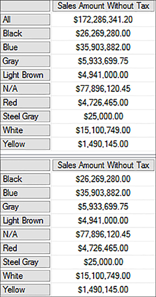
Let’s say that the business requirement is to show the total row after listing all the members. In that case, you can create a set of sets. The first set is the set of members using the Level syntax, and the second set is the All member. Both sets are enclosed in braces to create the outer set. Listing 3-11 shows you how to construct a set of sets and Figure 3-17 shows the results of executing this query.
LISTING 3-11 MEMBERS function in a set of sets
SELECT
[Measures].[Sales Amount Without Tax] ON COLUMNS,
{[Stock Item].[Color].[Color].Members, [Stock Item].[Color].[All]} ON ROWS
FROM
[Wide World Importers DW];

A common analytical requirement is to sort the set of members in a sequence other than the order defined by the OrderBy property for the attribute. To apply a different sort order to the members, you use the ORDER function. This function requires you to supply a minimum of two arguments, and optionally a third argument to specify a sort direction by using ASC or DESC for ascending or descending, respectively. The first argument is the set to sort and the second argument is the value by which to sort. If you omit the sort direction, the default behavior is to sort the set in ascending order. Listing 3-12 is a modification of the previous example in which the first set is sorted in descending order of sales. You can see the results in Figure 3-18.
SELECT
[Measures].[Sales Amount Without Tax] ON COLUMNS,
{
ORDER(
[Stock Item].[Color].[Color].Members,
[Measures].[Sales Amount Without Tax],
DESC),
[Stock Item].[Color].[All]
} ON ROWS
FROM
[Wide World Importers DW];

The value that you use as the second argument is not required to be returned in the query results, nor must it be a numeric value. Furthermore, you can display a subset of the results by nesting the results of the ORDER function, which returns a set, inside the HEAD function, which takes a set or set expression as its first argument and the number of members to return from the beginning of the set as the second argument. As an example, the query in Listing 3-13 sorts stock items by profit in descending order to show the five most profitable items first, but the query returns the Sales Amount Without Tax measure. Notice that you can enclose multi-line comments between the /* and */ symbols to embed comments within a query as documentation of the steps performed. Comments are helpful when you have functions nested inside of functions. You can see the query results in Figure 3-19.
LISTING 3-13 ORDER function nested inside HEAD function
SELECT
[Measures].[Sales Amount Without Tax] ON COLUMNS,
HEAD(
/* First argument – set of stock items sorted by profit
in descending order */
ORDER(
[Stock Item].[Stock Item].[Stock Item].Members,
[Measures].[Profit],
DESC),
/* Second argument – specify the number of members of set
in first argument to return */
5)
ON ROWS
FROM
[Wide World Importers DW];

This example is also good for reviewing what happens when the SSAS formula engine processes the query. Remember that the first steps are to resolve the members to place on columns and rows. There is only one measure on columns, Sales Amount Without Tax, which is explicitly stated and does not require any further processing by the formula engine.
On the other hand, the set to place on rows does require processing. The following steps must occur before the tuples are constructed to return the values that you see in the measure column:
1. Specifically, the formula engine starts by resolving the ORDER function. It constructs a tuple for the measure in the second argument, Profit, and each member in the ORDER function’s first argument, the set of members on the Stock Item level of the Stock Item attribute hierarchy in the Stock Item dimension. That is, all members except the All member. The tuple also includes the WHERE clause in the query, if one exists.
2. The formula engine then retrieves the value for each of those tuples and sorts the members in descending order.
3. Next, the formula engine applies the HEAD function to reduce the set of all sorted members to the first five members, which are placed on rows.
4. The final step is to compute the tuples for each cell resulting from the intersections of rows and columns and return the results.
Important Understand the role of tuple construction in query processing
The steps required to construct tuples for query results is one of the most important concepts to understand about MDX query processing. Axis resolution is completely separate from the final step of retrieving values that you see returned in the query results.
MDX includes a shortcut function to achieve the same result, TOPCOUNT. This function takes three arguments: a set of members, the number of members to return when resolving the TOPCOUNT function, and an expression to use for sorting purposes. The TOPCOUNT function automatically performs a descending sort. Listing 3-14 reproduces the previous example by replacing the combination of the HEAD and ORDER function with the more concise TOPCOUNT function. The query results match those returned for the query in Listing 3-13 and shown in Figure 3-19.
LISTING 3-14 TOPCOUNT function
SELECT
[Measures].[Sales Amount Without Tax] ON COLUMNS,
TOPCOUNT(
[Stock Item].[Stock Item].[Stock Item].Members,
5,
[Measures].[Profit])
ON ROWS
FROM
[Wide World Importers DW];
Sometimes there is no value in a cube cell location specified by a tuple. As a query developer, you decide whether the absence of data is important to the user. If it is not, you can remove a member from the set on rows or columns by placing the NON EMPTY keyword on either axis or both axes. Listing 3-15 includes two queries to demonstrate the difference between omitting and including this keyword. The SSAS formula engine applies the keyword as its final step in processing a query. That is, it places applicable members on axes, resolves the tuples for the intersections of each row and column, and then removes members from the designated axis. Figure 3-20 shows the results of executing these two queries.
LISTING 3-15 NON EMPTY keyword
//Without NON EMPTY on columns – Unknown row displays null value in each column
SELECT
[Measures].[Sales Amount Without Tax] ON COLUMNS,
BOTTOMCOUNT(
[Stock Item].[Stock Item].[Stock Item].Members,
5,
[Measures].[Profit])
ON ROWS
FROM
[Wide World Importers DW];
GO
//With NON EMPTY on columns – Unknown row removed in final processing step
SELECT
[Measures].[Sales Amount Without Tax] ON COLUMNS,
NON EMPTY BOTTOMCOUNT(
[Stock Item].[Stock Item].[Stock Item].Members,
5,
[Measures].[Profit])
ON ROWS
FROM
[Wide World Importers DW];

You can also remove members from an axis set before tuple construction begins. One way to do this is shown in Listing 3-16. In second query of this example, the NONEMPTY function operates like a filter by creating a tuple for each member of the set specified as the first argument with the measure specified as the second argument and then removing any member for which the tuple is empty, as you can see in the partial results shown in Figure 3-21. Often when you use the NONEMPTY function in a query instead of the NON EMPTY keyword, the query performance is better because there are fewer tuples to resolve in the final step of query resolution.
LISTING 3-16 NONEMPTY function
// Without NONEMPTY function
SELECT
[Measures].[Sales Amount Without Tax] ON COLUMNS,
[City].[City].[City].Members ON ROWS
FROM
[Wide World Importers DW];
GO
// With NONEMPTY function
SELECT
[Measures].[Sales Amount Without Tax] ON COLUMNS,
NONEMPTY([City].[City].[City].Members, [Measures].[Sales Amount Without Tax])
ON ROWS
FROM
[Wide World Importers DW];

Another way to reduce the number of members in an axis set is to use the FILTER function. The FILTER function requires a set as its first argument and a Boolean expression that returns TRUE or FALSE as its second argument. You can optimize the query by using this function in combination with the NONEMPTY function to first remove the empty tuples before applying the filter, as shown in Listing 3-17. Here the query finds the City members with a value for Sales Amount Without Tax, creates a tuple for each City member and the measure in the second argument of the FILTER function, Sales Amount Without Tax, and compares the tuple’s value to the Boolean expression’s value, 400000. If the tuple is greater than 400000, the SSAS engine keeps that tuple’s City member in the axis set, as shown in Figure 3-22. Just as you can do with the ORDER function, you can reference a measure in the second argument of the FILTER function that is not returned on a query axis.
SELECT
[Measures].[Sales Amount Without Tax] ON COLUMNS,
FILTER(
NONEMPTY([City].[City].[City].Members, [Measures].[Sales Amount Without Tax]),
[Measures].[Sales Amount Without Tax] > 400000)
ON ROWS
FROM
[Wide World Importers DW];

Note FILTER function
The Boolean expression in the second argument of the FILTER function can combine multiple expressions by using AND or OR operators between conditions.
Another function with which you should be familiar is the DESCENDANTS function, which is both a set function and a navigation function although it is found only in the Sets folder in the query window’s function list. (Navigation functions are described in the next section of this chapter.) Whereas the functions explained earlier in this chapter have one syntax, there are multiple syntax options for the DESCENDANTS function. The first argument of the function can be a member expression or a set expression, the second argument can be a level expression or a numeric expression to specify a distance, and the third argument is an optional flag.
Listing 3-18 shows an example of using a member expression as the first argument and a level as the second argument. Consider the member expression as the starting point for navigating through a user-defined hierarchy to find a set of members. In this case, the starting point is CY2015, which is on the Calendar Year level. The SSAS engine then returns the members on the specified level, Calendar Month, that are associated with CY2015, as shown in Figure 3-23.
LISTING 3-18 DESCENDANTS function with member and level expressions
SELECT
[Measures].[Sales Amount Without Tax] ON COLUMNS,
DESCENDANTS(
[Invoice Date].[Calendar].[Calendar Year]. [CY2015],
[Invoice Date].[Calendar].[Calendar Month])
ON ROWS
FROM
[Wide World Importers DW];

You can add a flag to the function as a third argument to control whether to include members of other levels in the hierarchy path. Table 3-2 describes each of the available flags. Examples of queries using these flags and comments describing query results are shown in Listing 3-19.

LISTING 3-19 DESCENDANTS function with flag
// SELF - Returns only members of Month level subordinate to CY2015
// e.g. CY2015-Jan to CY2015-Dec
SELECT
[Measures].[Sales Amount Without Tax] ON COLUMNS,
DESCENDANTS(
[Invoice Date].[Calendar].[Calendar Year].[CY2015],
[Invoice Date].[Calendar].[Calendar Month],
SELF)
ON ROWS
FROM
[Wide World Importers DW];
GO
// AFTER - Returns only members of Date level subordinate to CY2015
// e.g. 2015-01-01 to 2015-12-31
SELECT
[Measures].[Sales Amount Without Tax] ON COLUMNS,
DESCENDANTS(
[Invoice Date].[Calendar].[Calendar Year].[CY2015],
[Invoice Date].[Calendar].[Calendar Month],
AFTER)
ON ROWS
FROM
[Wide World Importers DW];
GO
// BEFORE - Returns members of Year level above Calendar Month related to CY2015
// e.g. CY2015
SELECT
[Measures].[Sales Amount Without Tax] ON COLUMNS,
DESCENDANTS(
[Invoice Date].[Calendar].[Calendar Year].[CY2015],
[Invoice Date].[Calendar].[Calendar Month],
BEFORE)
ON ROWS
FROM
[Wide World Importers DW];
GO
// BEFORE_AND_AFTER - Returns members of Date level subordinate to CY2015 and
// Year level above Calendar Month related to CY2015
// e.g. CY2015 and 2015-01-01
SELECT
[Measures].[Sales Amount Without Tax] ON COLUMNS,
DESCENDANTS(
[Invoice Date].[Calendar].[Calendar Year].[CY2015],
[Invoice Date].[Calendar].[Calendar Month],
BEFORE_AND_AFTER)
ON ROWS
FROM
[Wide World Importers DW];
GO
// SELF_AND_AFTER - Returns members of Month level subordinate to CY2015 and
// members of Date level subordinate to CY2015
// e.g. CY2015-Jan to CY2015-Dec and 2015-01-01 to 2015-12-31 with
// Date members displayed below its parent Month member
SELECT
[Measures].[Sales Amount Without Tax] ON COLUMNS,
DESCENDANTS(
[Invoice Date].[Calendar].[Calendar Year].[CY2015],
[Invoice Date].[Calendar].[Calendar Month],
SELF_AND_AFTER)
ON ROWS
FROM
[Wide World Importers DW];
GO
// SELF_AND_BEFORE - Returns members of Month level subordinate to CY2015 and
// Year level above Calendar Month related to CY2015
// e.g. CY2015 and CY2015-Jan to CY2015-Dec
SELECT
[Measures].[Sales Amount Without Tax] ON COLUMNS,
DESCENDANTS(
[Invoice Date].[Calendar].[Calendar Year].[CY2015],
[Invoice Date].[Calendar].[Calendar Month],
SELF_AND_BEFORE)
ON ROWS
FROM
[Wide World Importers DW];
GO
// SELF_BEFORE_AFTER - Returns members of Date, Month levels subordinate to CY2015 and
// Year level above Calendar Month related to CY2015
// e.g. CY2015 and CY2015-Jan to CY2015-Dec and 2015-01-01 to 2015-12-31 with
// Date members displayed below its parent Month member and
// Year member displayed above all members
SELECT
[Measures].[Sales Amount Without Tax] ON COLUMNS,
DESCENDANTS(
[Invoice Date].[Calendar].[Calendar Year].[CY2015],
[Invoice Date].[Calendar].[Calendar Month],
SELF_BEFORE_AFTER)
ON ROWS
FROM
[Wide World Importers DW];
GO
// LEAVES - Returns members of Date level subordinate to CY2015
// e.g. 2015-01-01 to 2015-12-31
SELECT
[Measures].[Sales Amount Without Tax] ON COLUMNS,
DESCENDANTS(
[Invoice Date].[Calendar].[Calendar Year].[CY2015],,
LEAVES)
ON ROWS
FROM
[Wide World Importers DW];
GO
When you use a set expression as the first argument of the DESCENDANTS function, the SSAS engine processes each member in the set individually using the remaining arguments and then combines the results. In Listing 3-20, the set expression returns CY2015 and CY2016. Notice the use of distance as the second argument instead of specifying a level. Consequently, because each member in the set expression result is on the Calendar Year level, the members returned by the DESCENDANTS function are two levels lower on the Date level, 2015-01-01 to 2016-12-31.
LISTING 3-20 DESCENDANTS function with set expression and distance
// Returns members of Date level subordinate to CY2015 and CY2016
// e.g. 2015-01-01 to 2016-12-31
SELECT
[Measures].[Sales Amount Without Tax] ON COLUMNS,
DESCENDANTS(
// Set expression
TAIL(
NONEMPTY([Invoice Date].[Calendar].[Calendar Year].Members,
[Measures].[Sales Amount Without Tax])
, 2),
// Distance from member in first argument
2)
ON ROWS
FROM
[Wide World Importers DW];
Note DESCENDANTS function reference
For more information about the nuances of the DESCENDANTS function, refer to “Descendants (MDX)” at https://msdn.microsoft.com/en-us/library/ms146075.aspx.
Navigation functions
Most of the functions in the Navigation folder on the Functions tab of the metadata pane return a set of members or a single member that is related to a specified member within a hierarchy tree. The type of relationship between members on different levels is expressed using family terms, such as parent, child, siblings, or ancestor. Descendants is also a valid term to describe relationships, but this function appears in the Set folder as described earlier in this chapter.
Some navigation functions return a single member, such as the PARENT function. Other navigation functions return a set of members, such as CHILDREN. Listing 3-21 provides an example of these two functions. The PARENT function returns the member one level above the specified member, whereas the CHILDREN function returns a set of members one level below it.
LISTING 3-21 PARENT and CHILDREN functions
// Returns a member on the Calendar Year level, CY2016, and
// members of Date level subordinate to ISO Week 1 in CY2016, 2016-01-04 to 2016-01-10
SELECT
[Measures].[Sales Amount Without Tax] ON COLUMNS,
{ [Invoice Date].[ISO Calendar].[ISO Week Number].&[2016]&[1].PARENT,
[Invoice Date].[ISO Calendar].[ISO Week Number].&[2016]&[1].CHILDREN }
ON ROWS
FROM
[Wide World Importers DW];
Another commonly used navigation function is ANCESTOR, which you use to return a member at some level above the level on which the member’s parent is found. Like the DESCENDANTS function, you can specify either the level by name or by distance, as shown in Listing 3-22.
LISTING 3-22 ANCESTOR function
// Returns a member on the Calendar Year level, CY2016
// Specify level by name
SELECT
[Measures].[Sales Amount Without Tax] ON COLUMNS,
ANCESTOR([Invoice Date].[Calendar].[Date].[2016-01-01],
[Invoice Date].[Calendar].[Calendar Year])
ON ROWS
FROM
[Wide World Importers DW];
GO
// Specify level by distance
SELECT
[Measures].[Sales Amount Without Tax] ON COLUMNS,
ANCESTOR([Invoice Date].[Calendar].[Date].[2016-01-01], 2)
ON ROWS
FROM
[Wide World Importers DW];
You can also navigate between members on the same level. Use the SIBLINGS function to return members sharing the same parent or use PREVMEMBER or NEXTMEMBER to return members that are sequenced together (according to the OrderBy property for the attribute), as shown in Listing 3-23.
LISTING 3-23 SIBLINGS, PREVMEMBER, and NEXTMEMBER functions
// Returns dates that are children of CY2016-Jan, 2016-01-01 to 2016-01-31
SELECT
[Measures].[Sales Amount Without Tax] ON COLUMNS,
[Invoice Date].[Calendar].[Date].[2016-01-01].SIBLINGS
ON ROWS
FROM
[Wide World Importers DW];
GO
// Returns dates preceding and following 2016-01-01, 2015-12-31 and 2016-01-02
SELECT
[Measures].[Sales Amount Without Tax] ON COLUMNS,
{[Invoice Date].[Calendar].[Date].[2016-01-01].PREVMEMBER,
[Invoice Date].[Calendar].[Date].[2016-01-01].NEXTMEMBER}
ON ROWS
FROM[Wide World Importers DW];
Time functions
Time series analysis is often a business requirement that drives the development of a multidimensional database. MDX time functions make it easy to compare values with one point in time to other points in time, or to report cumulative values for a specified period of time.
Three of the functions available in the Time folder on the Functions page of the metadata pane return a member relative in time to the specified member, OPENINGPERIOD, CLOSINGPERIOD, and PARALLELPERIOD. The OPENINGPERIOD and CLOSINGPERIOD functions have a similar syntax. The first argument specifies the level on which the member to return is found, and the optional second argument is the parent of the member to return. The OPENINGPERIOD function returns the member that is first in the set of descendants for the specified member while the CLOSINGPERIOD function returns the last member in that set. For example, as you can see in Listing 3-24, you can use the CLOSINGPERIOD function to find the last day of the specified month. If you replace the second argument with a member of the Calendar Year level, the function returns the last day of the specified year.
LISTING 3-24 CLOSINGPERIOD function
// Returns last date member that is a descendant of CY2016-Feb, 2016-02-29
SELECT
[Measures].[Sales Amount Without Tax] ON COLUMNS,
CLOSINGPERIOD( [Invoice Date].[Calendar].[Date],
[Invoice Date].[Calendar].[CY2016-Feb] )
ON ROWS
FROM
[Wide World Importers DW];
GO
// Returns last date member that is a descendant of CY2015, 2015-12-31
SELECT
[Measures].[Sales Amount Without Tax] ON COLUMNS,
CLOSINGPERIOD( [Invoice Date].[Calendar].[Date],
[Invoice Date].[Calendar].[CY2015])
ON ROWS
FROM
[Wide World Importers DW];
The PARALLELPERIOD function is useful for retrieving a point in time that is the same distance from the beginning of a parallel time period as a specified member. For example, if you specify the second month of a quarter, such as May, you can use this function to get the second month of the previous quarter, which is February. From an annual perspective, May 2016 is the fifth month of the year, so you can request the fifth month of the previous year, or May 2015. You are not limited to retrieving a member from a previous quarter or year, but you can also specify the distance to a previous period to retrieve or even request a point in time in the future, as you can see in Listing 3-25.
LISTING 3-25 PARALLELPERIOD function
// Returns month in same position of prior year, CY2015-May
SELECT
[Measures].[Sales Amount Without Tax] ON COLUMNS,
PARALLELPERIOD(
// The level by which to determine parallelism
[Invoice Date].[Calendar].[Calendar Year],
// The number of periods to traverse
1,
[Invoice Date].[Calendar].[CY2016-May])
ON ROWS
FROM
[Wide World Importers DW];
GO
// Returns date in same position of prior month, 2016-04-15
SELECT
[Measures].[Sales Amount Without Tax] ON COLUMNS,
PARALLELPERIOD(
[Invoice Date].[Calendar].[Calendar Month],
1,
[Invoice Date].[Calendar].[2016-05-15])
ON ROWS
FROM
[Wide World Importers DW];
GO
// Returns date in same position of three months prior, 2016-02-15
SELECT
[Measures].[Sales Amount Without Tax] ON COLUMNS,
PARALLELPERIOD(
[Invoice Date].[Calendar].[Calendar Month],
3,
[Invoice Date].[Calendar].[2016-05-15])
ON ROWS
FROM
[Wide World Importers DW];
GO
// Returns month in same position of next year, CY2016-Jan
SELECT
[Measures].[Sales Amount Without Tax] ON COLUMNS,
PARALLELPERIOD(
[Invoice Date].[Calendar].[Calendar Year],
-1,
[Invoice Date].[Calendar].[CY2015-Jan])
ON ROWS
FROM
[Wide World Importers DW];
The remaining time functions return sets. The generic function PERIODSTODATE is useful for generating a set of siblings for which the first member in the set is the first member in the period, and the last member is a member that is specified explicitly or dynamically. When you use this function to create a set to place on an axis, you explicitly define the last member of the set, as shown in Listing 3-26. However, when you use the PERIODSTODATE function in an expression that returns a value in a manner similar to the use of the YTD function demonstrated in the “Query-scoped calculations” section of this chapter, the last member of the set depends on the tuple context.
LISTING 3-26 PERIODSTODATE function
// Returns a set of months from the beginning of the year to CY2016-Mar,
// CY2016-Jan to CY2016-Mar
SELECT
[Measures].[Sales Amount Without Tax] ON COLUMNS,
PERIODSTODATE(
// The level that determines the period of time to traverse
[Invoice Date].[Calendar].[Calendar Year],
// The last member of the set to return
[Invoice Date].[Calendar].[CY2016-Mar])
ON ROWS
FROM
[Wide World Importers DW];
GO
// Returns a set of dates from the beginning of the ISO Week to 2016-03-24,
// 2016-03-21 to 2016-03-24
SELECT
[Measures].[Sales Amount Without Tax] ON COLUMNS,
PERIODSTODATE(
[Invoice Date].[ISO Calendar].[ISO Week Number],
[Invoice Date].[ISO Calendar].[2016-03-24])
ON ROWS
FROM
[Wide World Importers DW];
Query-scoped calculations
Ideally, you add frequently-used calculations to a cube as described in Skill 3.2, “Implement custom MDX solutions,” but there might be situations requiring you to create query-scoped calculations. A query-scoped calculation is a calculation that is evaluated at query time and does not persist in SSAS for reuse in subsequent queries. One reason to create a query-scoped calculation is to test logic prior to adding it permanently to the cube. Another reason is to support dynamic logic that is dependent on information available only at query time, such as parameter selections by a user that an application includes in the construction of an MDX query.
When you create a query-scoped calculation, you define either a member expression (also known as a calculated member), or a set expression by adding a WITH clause before the SELECT clause in a query. You can then use the new member or set in an expression that you use to create another member or set in the WITH clause or place on an axis, as shown in Listing 3-27. You can also reference the member in the query’s WHERE clause. You can define the formatting for a measure by adding a comma and the FORMAT_STRING property to the end of the measure definition. Any format string that you can add here in the cube designer is valid. You can see the results of the Average Sales Amount calculation in Figure 3-24.
Note FORMAT_STRING property
By default, the format string definition applies only to non-zero measure values. You can add sections to define formatting for nulls, zeros, and empty strings. To learn more, see “FORMAT_STRING Contents (MDX)” at https://msdn.microsoft.com/en-us/library/ms146084.aspx.
LISTING 3-27 Member and set definitions as query-scoped calculations
WITH
MEMBER [Measures].[Average Sales Amount] AS
[Measures].[Sales Amount Without Tax] / [Measures].[Quantity],
FORMAT_STRING = "Currency"
SET [Small Stock Items] AS
{[Stock Item].[Size].&[3XS],
[Stock Item].[Size].&[S],
[Stock Item].[Size].&[XS],
[Stock Item].[Size].&[XXS]}
SELECT
{[Measures].[Sales Amount Without Tax],
[Measures].[Quantity],
[Measures].[Average Sales Amount]} ON COLUMNS,
[Small Stock Items] ON ROWS
FROM
[Wide World Importers DW];

You can define multiple member or set expressions in the WITH clause. After using the SET or MEMBER keyword, you supply a name for the query-scoped calculation, follow the name with the keyword AS, and then add an expression that returns a set or tuple, respectively. When the member you create is a measure, prefix the member name with [Measures] and a period. This use of a WITH clause is much different in MDX than in T-SQL.
Statistical functions
You can also create a member as part of non-measure dimension in the cube, in which case you must provide the name of a dimension and a hierarchy in addition to the name of an existing member for which the calculated member becomes a child member. As an example, you might create a calculated member as a placeholder in a dimension for a value derived by using one of the functions in the Statistical folder on the Functions pane, such as AGGREGATE or SUM. This technique is analogous to creating a formula in Excel that references multiple cells to derive a new value that displays in a separate cell.
With a few exceptions, the functions in this group take a set as the first argument, and optionally take a numeric expression as the second argument. You omit the second argument when creating a calculated member, as shown in Listing 3-28, because the numeric value is determined at query time when the tuple resolution process adds a measure. In this example, the AGGREGATE function is used to create a non-measure dimension member, which is shown in Figure 3-25.
LISTING 3-28 AGGREGATE function for calculated member
WITH
MEMBER [Measures].[Average Sales Amount] AS
[Measures].[Sales Amount Without Tax] / [Measures].[Quantity],
FORMAT_STRING = "Currency"
MEMBER [City].[Sales Territory].[All].[West] AS
AGGREGATE(
{[City].[Sales Territory].[Far West],
[City].[Sales Territory].[Southwest]})
SELECT
{[Measures].[Sales Amount Without Tax],
[Measures].[Average Sales Amount]}
ON COLUMNS,
{[City].[Sales Territory].[Far West],
[City].[Sales Territory].[Southwest],
[City].[Sales Territory].[West]}
ON ROWS
FROM
[Wide World Importers DW];

When you use a statistical function to create a calculated measure in a query, you must include the second argument. Consider Listing 3-29, in which the SUM function is used to define a YTD Sales measure. The tuple resolution process is more complex in this case. Consider the cell intersection of CY2016-Jan and YTD Sales. The YTD function instructs the SSAS engine to build a set that includes each month from the beginning of the year to the member on the current row, which is returned by the CURRENTMEMBER function. In this case, the set contains only one member, CY2016-Jan. That member is combined with the measure in the second argument of the SUM function to create a tuple and a value is returned as you see in Figure 3-26. In the next row, because the set contains both CY2016-Jan and CY2016-Feb, two tuples are created and then added together. This process is repeated for CY2016-Mar, which results in the creation of three tuples that are added together.
LISTING 3-29 SUM function for calculated measure
WITH
MEMBER [Measures].[YTD Sales] AS
SUM(YTD([Invoice Date].[Calendar].CURRENTMEMBER),
[Measures].[Sales Amount Without Tax])
SELECT
{[Measures].[Sales Amount Without Tax],
[Measures].[YTD Sales]}
ON COLUMNS,
{[Invoice Date].[Calendar].[CY2016-Jan],
[Invoice Date].[Calendar].[CY2016-Feb],
[Invoice Date].[Calendar].[CY2016-Mar]}
ON ROWS
FROM
[Wide World Importers DW];

Conditional expressions
A conditional expression is useful for testing cell values before performing division or dynamically changing the value returned by an expression on a tuple by tuple basis. When you set up a conditional expression, you specify a search condition that the SSAS engine evaluates at query time as either TRUE or FALSE. The condition can be defined by using comparison operators or logical functions that return TRUE or FALSE. If you have a simple search condition, you can use the IIF function. For multiple search conditions, you can use a instead. Listing 3-30 provides examples of your options for constructing conditional expressions and the results are shown in Figure 3-27.
LISTING 3-30 Conditional expressions
WITH
MEMBER [Measures].[A] AS NULL
MEMBER [Measures].[Division Error] AS
[Measures].[Sales Amount Without Tax] /
[Measures].[A]
MEMBER [Measures].[Division No Error] AS
IIF(
// Argument 1 - Logical function ISEMPTY, OR logic, equality comparison
ISEMPTY([Measures].[A]) OR [Measures].[A] = 0,
// Argument 2 - Value to return if Argument 1 is TRUE
NULL,
// Argument 3 - Value to return if Argument 1 is FALSE
[Measures].[Sales Amount Without Tax] /
[Measures].[A]
)
MEMBER [Measures].[Case Stmt] AS
CASE
WHEN [Stock Item].[Color].CurrentMember IS [Stock Item].[Color].[Blue]
THEN "Blue"
WHEN [Stock Item].[Color].CurrentMember IS [Stock Item].[Color].[Black]
THEN "Not Blue"
ELSE
"Other"
END
SELECT
{[Measures].[Sales Amount Without Tax],
[Measures].[Division Error],
[Measures].[Division No Error],
[Measures].[Case Stmt]}
ON COLUMNS,
TOPCOUNT([Stock Item].[Color].[Color].Members, 3, [Measures].[Sales Amount Without Tax])
ON ROWS
FROM
[Wide World Importers DW];

String functions
Not only can you explicitly define a string to return as a measure, but you can also generate a string by using functions found in the Strings folder in the Functions pane, such as SETTOSTR and STRTOMEMBER. This type of string function is helpful for troubleshooting MDX queries or building dynamic MDX queries in which you construct a reference to a member at query time.
In Listing 3-31, the Set Members measure first evaluates the contents of the set generated by the YTD function for the current row and then converts the set object to a string by using the SETTOSTR function, as you can see in Figure 3-28. If you fail to use the SETTOSTR function, you cannot see the set’s contents because a measure must be typed as a numeric value or a string. Furthermore, the members placed on the ROWS axis are determined at query time based on the current month, which means that your query results are different when you execute this query in a month other than January. The NOW function returns the current date and time, which the query converts to the first three characters of the month name by using the FORMAT function with the “MMM” argument. This truncated month name is concatenated strings to construct a valid unique name of a member for the first item in a set range. The last item appends the NEXTMEMBER function twice to return the month that is two months after the current month.
Note Supported VBA functions
In addition to NOW, MDX supports several other VBA functions. A complete list is available at “VBA functions in MDX and DAX” at https://msdn.microsoft.com/en-us/library/hh510163.aspx.
LISTING 3-31 SETTOSTR and STRTOMEMBER functions
WITH
MEMBER [Measures].[Set Members] AS
SETTOSTR(YTD([Invoice Date].[Calendar].CURRENTMEMBER))
SELECT
[Measures].[Set Members]
ON COLUMNS,
{
STRTOMEMBER("[Invoice Date].[Calendar].[CY2016-" + FORMAT(NOW(),"MMM") + "]") :
STRTOMEMBER("[Invoice Date].[Calendar].[CY2016-" + FORMAT(NOW(),"MMM") +
"]").NEXTMEMBER.NEXTMEMBER
}
ON ROWS
FROM
[Wide World Importers DW];

Some additional string functions are found in the Metadata folder in the Functions pane, such as NAME and UNQIUENAME. Listing 3-32 provides examples of each of these functions. You can use these functions for troubleshooting purposes or working with parameters for MDX queries in SSRS reports.
LISTING 3-32 NAME and UNIQUENAME functions
WITH
MEMBER [Measures].[Name Function] AS
[Invoice Date].[Calendar].CURRENTMEMBER.NAME
MEMBER [Measures].[UniqueName Function] AS
[Invoice Date].[Calendar].CURRENTMEMBER.UNIQUENAME
SELECT
{[Measures].[Name Function],
[Measures].[UniqueName Function]}
ON COLUMNS,
{[Invoice Date].[Calendar].[CY2016-Jan] :
[Invoice Date].[Calendar].[CY2016-Mar]
}
ON ROWS
FROM
[Wide World Importers DW];

Note MDX queries in SSRS
James Beresford describes how to work with UNIQUENAME in his article, “Passing Parameters to MDX Shared Datasets in SSRS” at http://www.bimonkey.com/2014/04/passing-parameters-to-mdx-shared-datasets-in-ssrs/.
Another useful string function is PROPERTIES, which you can find in the Navigation folder in the Functions pane. When you set an attribute’s AttributeHierarchyEnabled property to False, you can access the value of that attribute by using the PROPERTIES function, as shown in Listing 3-33. Figure 3-30 shows the value displayed as if it were a measure. Instead of retrieving a tuple from the cube, SSAS retrieves the value from dimension storage for each city returned on rows.
LISTING 3-33 PROPERTIES functions
WITH
MEMBER [Measures].[Latest Recorded Population] AS
[City].[City].PROPERTIES( "Latest Recorded Population" )
SELECT
{[Measures].[Latest Recorded Population]}
ON COLUMNS,
TOPCOUNT([City].[City].[City].Members, 3, [Measures].[Profit])
ON ROWS
FROM
[Wide World Importers DW];

An understanding of MDX objects is key to correct development of MDX queries and calculations. Be prepared to recognize definitions of MDX objects and to distinguish one object type from another. For example, you should clearly understand the difference between tuples and sets, recognize the syntax of these objects, and use them correctly in expressions.
Need More Review? MDX tutorial
A good online resource for learning MDX is Stairway to MDX developed by Bill Pearson and available at http://www.sqlservercentral.com/stairway/72404/.
Skill 3.2: Implement custom MDX solutions
There are multiple options for implementing MDX in a multidimensional database. In any given database, business requirements might not allow you to use all these options. However, you should be prepared for exam questions that test your familiarity with the options described in this section.
This section covers how to:
![]() Create custom MDX or logical solutions for pre-prepared case tasks or business rules
Create custom MDX or logical solutions for pre-prepared case tasks or business rules
Create custom MDX or logical solutions for pre-prepared case tasks or business rules
One benefit of using custom MDX in a cube is the centralization of business logic to ensure that common calculations are consistently performed. Another benefit of storing MDX calculations in a cube is the caching of calculation results by the SSAS formula engine. When one user executes a query that uses a calculation, it remains available for other queries to use, regardless of which applications send those queries to SSAS, so query performance can be faster for the subsequent queries.
You store calculations in a cube by updating the MDX script that is created when you define a new cube. The SSAS engine uses the MDX script to determine how to resolve the values for each cell in a cube. In other words, the MDX script determines whether a cell’s value is set by data loaded from a source table or by one or more calculations.
Calculated measures
Calculated measures, introduced in Skill 3.1, are calculated members that are assigned to the Measures dimension. You can test the logic of a calculated measure by defining it in the WITH clause of an MDX query that you execute in SSMS, and then add it permanently to the cube by creating a new calculated member on the Calculations tab of the cube designer, as described in Chapter 1. The example in Chapter 1 described how to use the Form View to add the Profit Margin Percent calculation.
You can also create a new calculated measure by using the Script View and adding code to the MDX script. In SSDT, open the 70-768-Ch1 solution, open the Wide World Importers DW cube, click the Calculations tab, and click the Script View button on the cube designer’s toolbar. The MDX script currently contains two commands, shown in Listing 3-34: CALCULATE and CREATE MEMBER.
Note Import SSAS multidimensional project
If you do not have the 70-768-Ch1 solution from Chapter 1, but have restored the 70-768-Ch1.ABF file from the sample code files to your SSAS server, you can create a project from the restored database in SSDT. Point to New on the File menu, click Project, select Import From Server (Multidimensional And Data Mining), type a name for the project and solution, specify a location for the solution, and click OK. In the Import Analysis Services Database Wizard, click Next, select the 70-768-Ch1 database, click Next, and click Finish.
LISTING 3-34 MDX script with CALCULATE and CREATE MEMBER commands
/*
The CALCULATE command controls the aggregation of leaf cells in the cube.
If the CALCULATE command is deleted or modified, the data within the cube is affected.
You should edit this command only if you manually specify how the cube is aggregated.
*/
CALCULATE;
CREATE MEMBER CURRENTCUBE.[Measures].[Profit Margin Percent]
AS [Measures].[Profit]/[Measures].[Sales Amount Without Tax],
FORMAT_STRING = "Percent",
VISIBLE = 1 ;
Notice the warning that appears above the CALCULATE command explaining that this command controls the aggregation of cell values. If you remove this command, the only queries that return values are those that retrieve tuples at the bottom level of each attribute hierarchy, also known as the leaf level, which defeats the purpose of building a cube. A leaf-level cell is normally populated by loading data from a fact table, but can be overridden by an expression in the MDX script. The CALCULATE command instructs the SSAS engine to populate non-leaf cells with values derived by aggregating cells from lower levels, regardless of the source of the cell values.
The addition of the calculated measure in Chapter 1 by using the Form View added the CREATE MEMBER command to the MDX script. The syntax of the CREATE MEMBER command is similar to the definition of a calculated measure in a query-scoped calculation as described in Skill 3.1, but it includes the addition of a reference to the cube to which the member is added. In this case, the reference is to CURRENTCUBE.
For a full description of all available arguments for this command, see “CREATE MEMBER Statement (MDX)” at https://msdn.microsoft.com/en-us/library/ms144787.aspx.
Skill 3.1 introduced many different ways to build a measure by using tuples that rely on the current context of members on rows, columns, or the WHERE clause. Another technique with which you should be familiar is the use of a tuple to override the current context. A common calculation requiring this behavior is a percent of total, such as the one shown in Listing 3-35. This code also demonstrates the use of two new properties: FORE_COLOR and ASSOCIATED_MEASURE_GROUP. The FORE_COLOR property requires an expression, either static or conditional, that sets the text of a cell to a color in the Microsoft Windows operating system red-green-blue (RGB) format, such as 32768 for green and 0 for black. (A color picker is available in Form View to alleviate the need to find RGB numbers.) The ASSOCIATED_MEASURE_GROUP property links the calculation to a specific measure group. A client tool can use this information to display the calculated measure in the same folder as non-calculated members, but bear in mind that some client tools ignore this metadata.
LISTING 3-35 MDX script with calculated measure for percent of total
CREATE MEMBER CURRENTCUBE.[Measures].[Percent of Buying Group Sales Total]
AS [Measures].[Sales Amount Without Tax] /
([Measures].[Sales Amount Without Tax],[Customer].[Buying Group].[All] ),
FORMAT_STRING = "Percent",
FORE_COLOR = IIF([Measures].[Percent of Buying Group Sales Total] > 0.35, 32768
/*Green*/, 0 /*Black*/),
VISIBLE = 1 ,
ASSOCIATED_MEASURE_GROUP = 'Sale' ;
Add the code in Listing 3-35 to the MDX script, and then deploy the project to update the server with the new calculated measure. To test it, click the Browser tab of the cube designer, click Analyze In Excel on the Cube menu, click Enable in the security warning dialog box, and then select the following check boxes in the PivotTable Fields list: Sales Amount Without Tax, Percent Of Buying Group Sales Total, and Customer.Buying Group. The Microsoft Excel Security Notice displays a warning before opening the workbook because it contains an external data connection. In this case, the external data connection is trusted because it is generated in response to your selection of the Analyze In Excel command in the cube designer. You cannot view your cube in an Excel PivotTable unless you respond to the warning by clicking Enable.
Note CREATE MEMBER syntax
For a full description of all available arguments for this command, see “CREATE MEMBER Statement (MDX)” at https://msdn.microsoft.com/en-us/library/ms144787.aspx.
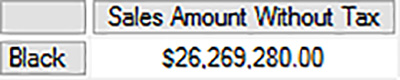
The resulting pivot table, shown in Figure 3-31, displays the sales amount and percentage contribution of each buying group. Furthermore, the value for the N/A row is displayed in a green font due to the conditional formatting instruction in the calculated measure definition.

The SSAS engine breaks down the Percent of Buying Group Sales Total calculation into two steps. First, it constructs a tuple for the numerator by combining the Sales Amount Without Tax measure with other dimension members to shape the context of the query. For example, in row 2 of Figure 3-31, the numerator tuple is ([Measures].[Sales Amount Without Tax], [Customer].[Buying Group].[Tailspin Toys]). Second, the SSAS engine constructs the denominator tuple, ([Measures].[Sales Amount Without Tax], [Customer].[Buying Group].[All]). This query includes no other dimension members to include in the tuple. In addition, the presence of the [Customer].[Buying Group].[All]) member overrides the inclusion of the [Customer].[Buying Group].[Tailspin Toys] member in the denominator’s tuple.
Calculated members
Of course, you can also add non-measure calculated members to a cube, such as the West member described in Skill 3.1, either in Script View by using the CREATE MEMBER command, or in Form View by using the graphical interface. To use Form view, perform the following steps:
1. Click the Form View button on the Calculations page of the cube designer in SSDT, and then click the New Calculated Member button.
2. In the Name box, type West.
3. In the Parent Hierarchy drop-down list, expand City, click Sales Territory, and click OK.
4. Next, click the Change button, click All, and click OK.
5. In the Expression box, type the following expression:
AGGREGATE(
{[City].[Sales Territory].[Far West],
[City].[Sales Territory].[Southwest]})
6. Deploy the project to add the new calculated member.
7. Click the Browser tab of the cube designer, click Analyze In Excel on the Cube menu, and click Enable in the security warning dialog box.
8. Select the following check boxes in the PivotTable Fields list: Sales Amount Without Tax, Profit, Profit Margin Percent, and Sales Territory in the City dimension.
You can see the West member listed after the Sales Territory members, as shown in Figure 3-32, with its value in the Sales Amount Without Tax and Profit columns calculated by summing Far West and Southwest values in the respective columns. Its value in the Profit Margin Percent column is calculated by first summing the Profit values for Far West and Southwest and then dividing by the sum of the Sales Amount Without Tax for those members. The use of the AGGREGATE function for non-measure calculated members ensures the proper calculation for each intersecting measure in a query.

In this example, Excel applied the format string correctly to the Profit Margin Percent value of the calculated member, but not to the Sales Amount Without Tax or Profit measures. You can fix this behavior by adding a LANGUAGE property to the CREATE MEMBER command as shown in Listing 3-36. In this example, 1033 is the locale ID value for United States English. You must add this property in Script View, because there is no graphical interface for configuring this property in Form View.
LISTING 3-36 LANGUAGE property for calculated member
CREATE MEMBER CURRENTCUBE.[City].[Sales Territory].[All].West
AS AGGREGATE(
{[City].[Sales Territory].[Far West],
[City].[Sales Territory].[Southwest]}),
VISIBLE = 1,
LANGUAGE = 1033 ;
Note Locale ID values
You can find a complete list of locale ID values in “Microsoft Locale ID Values” at https://msdn.microsoft.com/en-us/library/ms912047.aspx.
Named sets
Just as you can add a set to the WITH clause, you can add an object called a named set to a cube for sets that are commonly queried by users. However, as part of the definition of a named set, you must also specify whether the set is dynamic or static, as shown in Listing 3-37. The two set definitions in this listing are identical, except the type of set, dynamic or static, is stated after the CREATE command. With a dynamic named set, the members of the set can change at query time based on the current context of objects on axes and in the WHERE clause. By contrast, a static named set always returns the same set members regardless of changes to query context. In SSDT, switch to Script View and add the code in Listing 3-37 to the MDX script.
LISTING 3-37 MDX script for dynamic and static named sets
CREATE DYNAMIC SET CURRENTCUBE.[Top 3 Stock Items Dynamic]
AS TOPCOUNT
(
[Stock Item].[Stock Item].[Stock Item].Members,
3,
[Measures].[Sales Amount Without Tax]
),
DISPLAY_FOLDER = 'Stock Item Sets' ;
CREATE STATIC SET CURRENTCUBE.[Top 3 Stock Items Static]
AS TOPCOUNT
(
[Stock Item].[Stock Item].[Stock Item].Members,
3,
[Measures].[Sales Amount Without Tax]
),
DISPLAY_FOLDER = 'Stock Item Sets' ;
Next, test the changes by following these steps:
1. Deploy the project, click the Browser tab of the cube designer, click Analyze In Excel on the Cube menu, and click Enable in the security warning dialog box.
2. Select the Sales Amount Without Tax check box in the PivotTable Fields list. Scroll down in the list to locate the Stock Item dimension, expand the Stock Item Sets folder, and select the Top 3 Stock Items Static check box to create the pivot table shown in Figure 3-33.

3. Now expand the More Fields folder in the Invoice Date dimension and drag Invoice Date.Calendar year to the Filters pane below the PivotTable Fields list.
4. In the pivot table, select CY2013 in the Invoice Date.Calendar year drop-down list. Notice the values in the Sales Amount Without Tax column change, but the three stock items in column A remain the same. A static named set retains the same members in the set regardless of changes to the query context. Therefore, in this example, the static Top 3 Stock Items Static named set represents the top three stock items for all dates, all customers, all sales territories, and so on.
5. Scroll back to the Stock Item Sets folder, clear the Top 3 Stock Items Static check box, and select the Top 3 Stock Items Dynamic check box. Notice the pivot table now displays different stock items, as shown in Figure 3-34. If you change the Invoice Date.Calendar Year filter’s selection from CY2013 to CY2015, the first member in the set changes. Moreover, as you add more filters to the pivot table, you see different combinations of members in the pivot table. A dynamic set factors in the query context.

In this example in which the TOPCOUNT function determines which members are added to the set, the tuple used as the third argument is no longer [Measures].[Sales Amount Without Tax]. It instead includes the query’s rows, columns, or WHERE clause for any dimension not named in the first argument of the function. To produce the set shown in Figure 3-34, the tuple for which the stock item members are sorted and filtered to the top three is ([Measures].[Sales Amount Without Tax], [Invoice Date].[Calendar Year].[CY2013]).
Default member
If you do not explicitly define a default member for an attribute hierarchy, the SSAS engine treats the All member at the top level of the hierarchy as the default member. Remember that the SSAS engine includes the default member from each attribute hierarchy in each tuple generated as the final step of processing an MDX query if the attribute hierarchy does not appear on rows or columns or in the WHERE clause.
Let’s say that you want to set Far West as the default member for the Sales Territory attribute in the City dimension. To do this, follow these steps:
1. Open the dimension designer for City in SSDT and click Sales Territory in the Attributes pane on the Dimension Structure page.
2. In the Properties window, click the ellipsis button in the DefaultMember box.
3. In the Set Default Member – Sales Territory dialog box, click Choose A Member To Be The Default, expand All, click Far West(see Figure 3-35), and then click OK.

As an alternative, you can define the default member by using an MDX expression. The MDX expression can be a simple reference of a static member, such as [City].[Sales Territory].&[Far West]. The expression can also be a more complex dynamic expression by using functions like USERNAME or NOW to select a member based on the current user or date and time, to name two examples.
Note Use default members with caution
If you implement default members, be sure to educate users about its existence and the ability to override the default member at query time. The implementation of default members permanently applies a filter to an attribute hierarchy. Although a default member can be overridden in a query by requesting all members from the attribute hierarchy, an extra step is required from users which might not be intuitive.
Dimension and cell-level security
You can use MDX functions to define security and default members by role. Like tabular models, multidimensional models use role-based security to determine what users can see and do, although the implementation is quite different.
By default, when you deploy a multidimensional model to the server, no one can query it except you and the server administrators. At minimum, you must define a role and add Windows logins or groups to the role and grant read access to the cube. To do this in SSDT, right-click the Roles folder in Solution Explorer, and click New Role. In Solution Explorer, right-click the new role, Role.role, click Rename, and type a name for the role, such as Browsers.role, and click Yes to confirm. On the General page of the role designer, you can select any or all of the following database permissions for the role:
![]() Full Control (Administrator) This role has full permissions on the database. This selection allows a user to alter or delete the database, perform processing operations, and configure security.
Full Control (Administrator) This role has full permissions on the database. This selection allows a user to alter or delete the database, perform processing operations, and configure security.
![]() Process Database This role allows a user to perform processing operations by using SQL Server Integration Services (SSIS) or SSMS.
Process Database This role allows a user to perform processing operations by using SQL Server Integration Services (SSIS) or SSMS.
![]() Read Definition This role allows the user to script the database or to view metadata for database objects without granting the ability to modify the objects or read the data.
Read Definition This role allows the user to script the database or to view metadata for database objects without granting the ability to modify the objects or read the data.
When you want to create a role solely for the purpose of granting users the ability to browse or query a cube, leave the database permissions check boxes cleared perform the following steps:
1. Click the Membership tab of the role designer.
2. Click Add and then use the Select Users Or Groups dialog box to enter Windows logins or groups to the role. To follow the examples in this chapter, you do not need to assign any users to the role, because you can test a role with no users.
3. Next, click the Cubes tab of the role designer, and click Read in the Access drop-down list for the Wide World Importers DW cube.
If you were to deploy the project at this point, the role would enable its members to query the cube without further restriction. When you want to limit which dimension members that users can see, you can add dimension security by following these steps:
1. Click the Dimension Data tab in the role designer. By default, users can see all members in any attribute in any dimension. You can use the Dimension and Attribute Hierarchy drop-down lists on the Dimension Data page to target a specific attribute, and then select or clear check boxes to determine which dimension members that users can see or not see, respectively. As an alternative, click the Advanced tab to use MDX expressions to define allowed and denied member sets in addition to a default member. The default member defined for the role overrides the default member defined for the attribute in the dimension designer.
2. As an example, assume that you want to restrict users in the Browsers role to view data only for a subset of states in the City dimension. Specifically, you want users to see only the states that are associated with the Far West sales territory. In the Dimension drop-down list, click City and click OK.
3. Next, in the Attribute drop-down list, click State Province, and then click the Advanced tab. In the Allowed Member Set box, add the following set expression:
EXISTS(
[City].[State Province].[State Province].Members,
[City].[Sales Territory].[Far West]
)
Note Dimension security
When configuring dimension security, you can select the Enable Visual Totals check box if you want the total for a hierarchy to reflect the filtered value. In other words, the user can see the aggregated value for allowed members. If you do not enable visual totals, the user can see the grand total for all members, which usually does not match the total of allowed members.
You can find a more extensive explanation of dimension security options in “Grant custom access to dimension data (Analysis Services)” at https://msdn.microsoft.com/en-us/library/ms175366.aspx. Richard Lees has written “SSAS Dynamic Security” to explain the user of the USERNAME function to define allowed member sets and default members at http://richardlees.blogspot.com/2010/10/ssas-dynamic-security.html.
4. If there are specific measures for which you do not want users to see values, you can define cell-level security. Unlike dimension security for which you specify a set expression, you define Boolean expressions to specify which measures are visible when configuring cell-level security. Perhaps for the Browsers role you want users to see all measures except the Profit measure and the related Profit Margin Percent calculated measure. On the Cell Data tab of the role designer, select the Enable Read-contingent Permissions check box, and type the following expression in the Allow Reading Of Cell Content Contingent On Cell Security box:
NOT Measures.CurrentMember IS [Measures].[Profit]
Note Cell-level security
There are several different approaches to defining cell-level security besides the examples described in this chapter. For additional examples, see “Grant custom access to cell data (Analysis Services)” at https://msdn.microsoft.com/en-us/library/ms174847.aspx.
After configuring a role, deploy the project. You can then test the security configuration for that role by following these steps:
1. On the Browser page of the cube designer, click the Reconnect button, and then click the Change User button to the left of the Reconnect button.
2. In the Security Context – Wide World Importers DW dialog box, click Roles, select the Browsers check box, and click OK twice.
3. In the metadata pane, expand the City dimension, expand the State Province attribute, and expand the State Province level, as shown in Figure 3-36. The only states visible to members of this role are those that belong to the Far West territory. Although other states exist in the attribute, they do not display when browsing the dimension due to the security configuration.

4. Drag the State Province attribute to the query window. Then expand the Measures folder and drag the following measures to the query window to test measure security: Sales Amount Without Tax, Profit, and Profit Margin Percent. As shown in Figure 3-37, the values for Sales Amount Without Tax display, but the values for Profit and Profit Margin Percent do not. Remember that you defined cell security only for Profit. However, because you used the read contingent option, security also applies to any calculated measure related to Profit, such as Profit Margin Percent in this case.

Important Role-based security is additive
Analysis Services security permissions are additive, which is counterintuitive. If a user is a member of two roles and one role grants permission to view data while another role removes permission, the permissions are combined and the user can view the data. You can read an in-depth article about this behavior in “The Additive Design of SSAS Role Security” at https://blogs.msdn.microsoft.com/psssql/2014/07/30/the-additive-design-of-ssas-role-security/.
Note Multidimensional model security architecture
This section provides only a high-level explanation of multidimensional model security. Although written for SQL Server 2008 R2, “User Access Security Architecture” at https://technet.microsoft.com/en-us/library/ms174927(v=sql.105).aspx remains applicable to SQL Server 2016 and provides more information about securing your multidimensional models.
Analysis Services Stored Procedures
The MDX language contains many more functions than those described earlier in this chapter. For the most part, MDX is capable of supporting most types of analysis that businesses commonly perform. When you need a specific operation to return a value, a string, or a set and none of the MDX functions meet your needs, you can create an Analysis Services stored procedure (ASSP) by creating and registering an assembly on the SSAS instance. As an example, financial analysis often requires an internal rate of return (IRR) calculation which might be easier to implement as a custom ASSP.
Unlike a SQL Server stored procedure that uses T-SQL to define an operation, an ASSP is implemented as a Microsoft Visual Basic .NET or C# assembly. Let’s say you have a developer in your organization that creates an assembly and sends it to you as a dynamic link library (DLL) file. You register the ASSP by following these steps:
1. In SSMS, connect to the SSAS multidimensional instance.
2. You then add the assembly to the server for use in any database or to a specific database if you want to limit the usage of the assembly’s functions. To do this, right-click the Assemblies folder for the server or expand a database’s folder and then right-click its Assemblies folder.
3. Next, click New Assembly. In the Register Server Assembly dialog box (or if you clicked New Assembly for a database, the Register Database Assembly dialog box), provide the following configuration information, as shown in Figure 3-38:
![]() Type Keep the default selection of .NET Assembly.
Type Keep the default selection of .NET Assembly.
![]() File name Type the path and assembly name in the text box or use the ellipsis button to navigate the file system and select the assembly.
File name Type the path and assembly name in the text box or use the ellipsis button to navigate the file system and select the assembly.
![]() Assembly name Type a name for the assembly.
Assembly name Type a name for the assembly.
![]() Include debug information If you select this check box, you can use the debugging feature in Visual Studio when executing a function in this assembly.
Include debug information If you select this check box, you can use the debugging feature in Visual Studio when executing a function in this assembly.
![]() Permissions Select one of the following options:
Permissions Select one of the following options:
![]() Safe Provides permission for internal computations.
Safe Provides permission for internal computations.
![]() External Access Provides permission for internal computations and access to external system resources, such as the file system or a database.
External Access Provides permission for internal computations and access to external system resources, such as the file system or a database.
![]() Unrestricted Provides no protections to the system.
Unrestricted Provides no protections to the system.
![]() Impersonation Set the code’s execution context for external resources by selecting one of the following options:
Impersonation Set the code’s execution context for external resources by selecting one of the following options:
![]() Use A Specific Windows User Name And Password Use a Windows login and password for a user authorized to access the external resource.
Use A Specific Windows User Name And Password Use a Windows login and password for a user authorized to access the external resource.
![]() Use The Service Account Assign the service account running the Analysis Services service to change the execution context for the code.
Use The Service Account Assign the service account running the Analysis Services service to change the execution context for the code.
![]() Use The Credentials Of The Current User Run the code under the Windows login for the current user.
Use The Credentials Of The Current User Run the code under the Windows login for the current user.
![]() Anonymous Assign the IUSER_servername Windows login user account as the execution context.
Anonymous Assign the IUSER_servername Windows login user account as the execution context.
![]() Default Default to running the code under the Windows login for the current user.
Default Default to running the code under the Windows login for the current user.

Let’s say that a hypothetical assembly, MyASSP.dll, includes a function named MyFunction that requires a measure as an argument and returns a value. To use this function after registering the assembly, you reference it by concatenating the assembly name, the function name, and the argument list, as shown in Listing 3-37.
SELECT
MyASSP.MyFunction([Measures].[A Measure])
ON COLUMNS
FROM [My Cube];
Note ASSP sample code
You can find several examples of ASSPs at “Analysis Services Stored Procedure Project” at https://asstoredprocedures.codeplex.com/.
 Exam Tip
You do not need to know how to develop an ASSP assembly for the exam. However, you should be familiar with the steps necessary to register the assembly and call the ASSP in an MDX query.
Define a SCOPE statement
You can restrict calculations in an MDX script not only to specific cells within a cube, but also to specific points at which the SSAS engine calculates cell values. To do this, you can use SCOPE statements and assignment operations in the MDX script. This capability allows you to implement complex business logic in a cube that is not possible with other types of calculated objects.
To better understand how to use SCOPE to implement complex business logic, consider the following requirements to calculate sales quotas for Wide World Importers:
![]() The monthly sales quota for CY2014 is a fixed amount for each month, $4,500,000.
The monthly sales quota for CY2014 is a fixed amount for each month, $4,500,000.
![]() The sales quota for CY2015 is calculated by multiplying the previous year’s sales by 110% and then equally allocating one-twelfth of this value to each month.
The sales quota for CY2015 is calculated by multiplying the previous year’s sales by 110% and then equally allocating one-twelfth of this value to each month.
Before creating the MDX script to apply these calculations, add a new measure to the cube by using the code shown in Listing 3-38. This CREATE MEMBER command defines the Sales Quota measure and assigns an initial value of NULL.
LISTING 3-38 Initialize the Sales Quota measure
CREATE MEMBER CURRENTCUBE.[Measures].[Sales Quota]
AS NULL,
VISIBLE = 1,
LANGUAGE = 1033;
Next, add code to the MDX script to allocate a fixed amount to each month in 2014. When the assignment of a value to a set of cells does not require multiple expressions, you can use an assignment operation, as shown in Listing 3-39. The left side of the equal sign, used as an assignment operator in an MDX script, is the portion of the cube to which the value on the right side of the assignment operator is assigned. This portion of the cube is known as a subcube.
LISTING 3-39 Assignment of a single value to a set of cells
([Invoice Date].[Calendar Year].[CY2014],
[Invoice Date].[Calendar].[Calendar Month].Members,
[Measures].[Sales Quota]) = 4500000;
A subcube always contains the All member of a hierarchy if no members of that hierarchy are explicitly defined. Otherwise, it can contain any of the following objects for a specified hierarchy:
![]() A single member of an attribute.
A single member of an attribute.
![]() Some or all members of a single level of an attribute or user-defined hierarchy.
Some or all members of a single level of an attribute or user-defined hierarchy.
![]() Descendants of a single member.
Descendants of a single member.
Your next step is to use a SCOPE statement to apply a series of MDX expressions to a subcube, as shown in Listing 3-40. By adding this code to the MDX script, you set the subcube defined as the argument for SCOPE as the target for every use of the THIS function until the END SCOPE statement is encountered. The FREEZE statement ensures that any statements subsequently added to the MDX script do not change the values assigned to the subcubes for CY2014 and CY2015.
LISTING 3-40 Equal allocation of prior year’s value to current year’s Calendar Month members
SCOPE([Invoice Date].[Calendar Year].[CY2015],
[Invoice Date].[Calendar].[Calendar Month].Members,
[Measures].[Sales Quota]);
THIS =
// create a tuple to retrieve sales one year prior
([Invoice Date].[Calendar].PARENT.PREVMEMBER,
[Measures].[Sales Amount Without Tax])
// multiply by 110%
* 1.1
// divide the result by 12 for equal allocation
/ 12;
END SCOPE;
FORMAT_STRING([Measures].[Sales Quota])= "Currency";
FREEZE;
Test the results of the new MDX script by following these steps:
1. Deploy the project, click the Browser tab of the cube designer, click Analyze In Excel on the Cube menu, and click Enable in the security warning dialog box.
2. Set up the pivot table by selecting the following check boxes: Sales Amount Without Taxes, Sales Quota, and Invoice Date.Calendar Month.
3. Drag the Calendar Month from the Columns pane to the Rows pane in the area below the PivotTable Fields list.
4. Drag Invoice Date.Calendar Year to the Filters pane, and select CY2014 in the Invoice Date.Calendar Year drop-down list.
5. Drag Sales Territory to the Filters pane, and select All in the Sales Territory drop-down list to produce the pivot table shown in Figure 3-39 in which you can see the fixed allocation of $4,500,000 to each month.

6. Now change the Invoice Date.Calendar Year filter to CY2015, as shown in Figure 3-40. Here the Sales Quota remains fixed across all months because it is an equal allocation. The allocation computation results from multiplying the CY2014 total sales amount of $49,929,487.20 by 110% which equals $54,922,435.90 and then dividing that value by 12. The result is $4,576,869.66.

Need More Review? MDX reference
A good online resource for learning MDX is Stairway to MDX developed by Bill Pearson and available at http://www.sqlservercentral.com/stairway/72404/.
Skill 3.3: Create formulas by using the DAX language
The DAX language is completely different from MDX and requires you to learn different skills and apply different through processes to develop appropriate queries and calculations. Whereas MDX functions work with members, sets, and hierarchies, DAX functions work with tables, columns, and relationships. Coverage of all DAX functions is out of scope for this book, but Skill 3.3 introduces you to the more commonly used functions and provides a solid foundation for applying key concepts as you learn similar types of functions.
This section covers how to:
![]() Use the EVALAUTE and CALCULATE functions
Use the EVALAUTE and CALCULATE functions
![]() Perform data analysis by using DAX
Perform data analysis by using DAX
Use the EVALUATE and CALCULATE functions
The 70-768 exam tests your ability to write DAX queries and work with functions, including CALCULATE, one of the most important functions. The ability to write DAX queries is also helpful for testing DAX formulas before you add them permanently to your tabular model as calculated measures just as you use MDX queries to test logic before adding calculated measures to a cube.
Note Sample database for this chapter
This chapter uses the database created in Chapter 2, “Design and publish a tabular model,” to illustrate DAX concepts and queries. However, if you have created this database, you should revert it to in-memory mode by changing the DirectQuery Mode property for the model to Off. You must process all tables in the model after changing the mode.
If you have not created this database, you can restore the ABF file included with this chapter’s code sample files. To do this, copy the 70-768-Ch2.ABF file from the location in which you stored the code sample files for this book to the Backup folder for your SQL Server instance, such as C:Program FilesMicrosoft SQL ServerMSAS13.TABULAROLAPBackup. Then open SQL Server Management Studio (SSMS), select Analysis Services in the Server Type drop-down list, provide the server name, and click Connect. In Object Explorer, right-click the Databases folder, and click Restore Database. In the Restore Database dialog box, click Browse, expand the Backup path folder, and select the 70-768-Ch2.ABF file, and click OK. In the Restore Database text box, type 70-768-Ch2, and click OK.
DAX query structure
The structure of a DAX query is much different from an MDX or T-SQL query. Listing 3-41 shows the simplest query that you can write in a client application such as SSMS. It contains an EVALUATE clause and the name of a table.
LISTING 3-41 Simplest DAX query
EVALUATE
'Stock Item'
Note Syntax for table names
If a table name contains an embedded space, reserved keywords, or characters outside the ANSI alphanumeric character range, you must enclose the name within single quotes.
To execute this query in SSMS, perform the following steps:
1. Connect to the tabular instance of SSAS, and then click the Analysis Services MDX Query button in the toolbar.
The MDX query window supports the execution of DAX queries, although you cannot use drag and drop to add objects from the metadata pane to the query window.
2. In the Available Databases drop-down list, select 70-768-Ch2, and then add the query shown in Listing 3-41.
3. Click Execute to see the query results, a portion of which is shown in Figure 3-41, although the rows you see might vary because the order of rows is not guaranteed with this query. In this case, the query returns every column and every row in the referenced table.
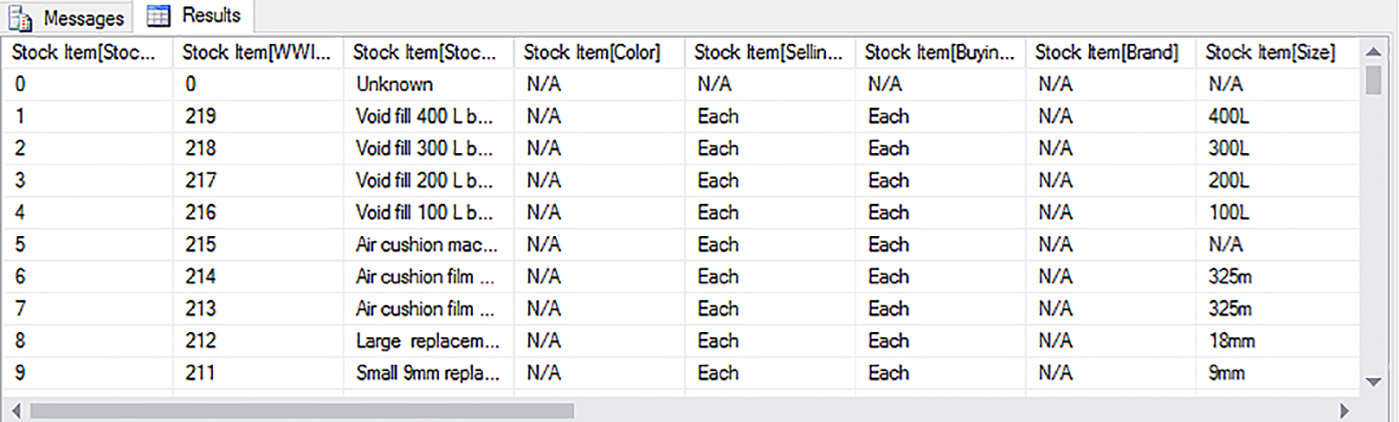
You can override the default sort order of the table by adding an ORDER BY clause, as shown in Listing 3-42. The ORDER BY clause contains a list of columns defining the sort order which is ascending by default. Only columns are permissible in this list; you cannot use expressions. The default sort order is ascending which you can make more explicit by appending the ASC keyword after the column name, Use the DESC keyword after the column name to reverse the sort direction, as shown in Figure 3-42.
LISTING 3-42 ORDER BY clause in DAX query
EVALUATE
'Stock Item'
ORDER BY
'Stock Item'[Color] DESC,
'Stock Item'[Size]
Note Syntax for unqualified and fully qualified column names
Sometimes you can use the unqualified name of a column in a query or in expressions. In that case, enclose the column name in brackets. However, a better practice is to use its fully qualified name to avoid ambiguity. Furthermore, some functions require you to do so. The fully qualified name of a column begins with its table name and ends with the column name.

To further refine the query results, you can add the optional START AT sub-clause inside the ORDER BY clause to specify the first row of the result set, as shown in Listing 3-43. Its primary purpose is to enable applications to display a limited set of data at a time, such as when an application allows users to page through data. Each argument in the START AT sub-clause defines the value for the corresponding column in the ORDER BY clause. In Listing 3-43, the value of “Red” in the START AT sub-clause corresponds to the Color column and “1/12 scale” corresponds to the Size column. A portion of the query results is shown in Figure 3-43.
LISTING 3-43 START AT sub-clause in DAX query
EVALUATE
'Stock Item'
ORDER BY
'Stock Item'[Color] DESC,
'Stock Item'[Size]
START AT
"Red",
"1/12 scale"

You control which rows and columns to return in the query’s result set by using a table expression rather than a table. A common way to return data from a tabular model in a query is to use the SUMMARIZE function. As shown in Listing 3-44, this function requires a table or table expression as its first argument and, at minimum, a pair of arguments for each column to summarize in the query results. This pair of arguments includes a string that becomes the name of the column in the query results and an expression to return a scalar value, as shown in Figure 3-44. In this example, the expressions for scalar values are references to measures defined in the tabular model. Notice that you can provide a column name that does not match the measure name. In addition, you can see how to use the FORMAT function to apply formatting to each measure.
Note FORMAT function
To see a list of permissible formats to use with the FORMAT function, see “Predefined Numeric formats for the FORMAT Function” at https://technet.microsoft.com/en-us/library/ee634561 and “Custom Numeric Formats for the FORMAT Function” at https://technet.microsoft.com/en-us/library/ee634206.
LISTING 3-44 SUMMARIZE function with two measures
EVALUATE
SUMMARIZE(
'Sale',
"Total Sales",
FORMAT('Sale'[Total Sales], "#,##0.00#"),
"Number of Sales Transactions",
FORMAT('Sale'[Sale Count], "#,#")
)
Note SUMMARIZECOLUMNS
A DAX function new to SQL Server 2016 is SUMMARIZECOLUMNS, which behaves similarly to SUMMARIZE, but uses slightly different syntax. You should experiment with the queries in this chapter by translating SUMMARIZE functions to SUMMARIZECOLUMNS. To learn more about working with this function, see “SUMMARIZECOLUMNS Function (DAX)” at https://msdn.microsoft.com/en-us/library/mt163696.aspx.
More often, you need a query to summarize results by groups, just like you can use a GROUP BY clause in a SQL statement. To do this, you can include a list of columns to use for grouping between the table name and the name/expression pairs, as shown in Listing 3-45. When you use columns from several tables, the relationships defined in the model ensure the values are summarized correctly. Remember that you can control the sort order of the results by using an ORDER BY clause.
LISTING 3-45 SUMMARIZE function with group by columns
EVALUATE
SUMMARIZE(
'Sale',
'Stock Item'[Color],
'Stock Item'[Brand],
"Total Sales",
'Sale'[Total Sales],
"Number of Sales Transactions",
'Sale'[Sale Count]
)
ORDER BY
'Stock Item'[Color]

If you want to include subtotals for each grouping, you can use the ROLLUP syntax as shown in Listing 3-46. In this example, because both columns used for grouping are included in the ROLLUP expression and the ORDER by clause. Subtotals for each color and for all colors appear in the query results, as shown in Figure 3-46. If you omit the ORDER BY clause, the subtotals appear after the row groups in the query results.
LISTING 3-46 SUMMARIZE function with ROLLUP
EVALUATE
SUMMARIZE(
'Sale',
ROLLUP(
'Stock Item'[Color],
'Stock Item'[Brand]
),
"Total Sales",
'Sale'[Total Sales],
"Number of Sales Transactions",
'Sale'[Sale Count]
)
ORDER BY
'Stock Item'[Color],
'Stock Item'[Brand]

Note SUMMARIZE function
For a full description of all the options available for using this function, see “SUMMARIZE Function DAX” at https://msdn.microsoft.com/en-us/library/gg492171.aspx. You can find a more in-depth review of its capabilities in Alberto Ferrari’s article, “All the secrets of SUMMARIZE,” at http://www.sqlbi.com/articles/all-the-secrets-of-summarize/.
Query-scoped measures
You can create a measure for use in a single query or to test in a query before adding it permanently to the tabular model in a query by adding a DEFINE clause prior to the EVALUATE clause, as show in Listing 3-47. In the DEFINE clause, you assign a name to a new measure and provide an expression, and then subsequently reference the measure in another new measure definition or in the EVALUATE clause. You can instead place the measure definition inline after the column name in the EVALUATE clause, but placing it in the DEFINE clause makes the query easier to read. You can see the results of this query in Figure 3-47.
DEFINE
MEASURE 'Sale'[Total Quantity] =
SUM('Sale'[Quantity])
MEASURE 'Sale'[Average Sales Amount] =
'Sale'[Total Sales] / 'Sale'[Total Quantity]
EVALUATE
SUMMARIZE(
'Sale',
'Stock Item'[Color],
"Total Sales",
'Sale'[Total Sales],
"Average Sales Amount",
'Sale'[Average Sales Amount]
)
ORDER BY
'Stock Item'[Color]

Important Measure name assignment
If you assign a new measure the same name as a measure in the tabular model, your new measure replaces the one in the model. For example, if your query defines a measure named [Total Sales], the value returned in the query results uses the query’s measure definition and does not use the calculation defined in the tabular model for [Total Sales]. However, if any other measure in the tabular model uses [Total Sales] to derive a value, that measure uses the tabular model’s definition for [Total Sales]. This behavior can be confusing. Therefore, you should strive to avoid reusing measure names in query-scoped measures.
One optimization technique that you can use when you add query-scoped measures is to separate the measure expression from the table returned by the SUMMARIZE function. You can do this by using the ADDCOLUMNS function, as shown in Listing 3-48. The first argument of this function is a table or expression that returns a table, and then subsequent arguments are name/expression pairs to append to the table. The execution of Listing 3-48 returns the same results shown in Figure 3-47.
LISTING 3-48 ADDCOLUMNS function to append query-scoped measures
DEFINE
MEASURE 'Sale'[Total Quantity] =
SUM('Sale'[Quantity])
MEASURE 'Sale'[Average Sales Amount] =
'Sale'[Total Sales] / 'Sale'[Total Quantity]
EVALUATE
ADDCOLUMNS(
SUMMARIZE(
'Sale',
'Stock Item'[Color]
),
"Total Sales",
'Sale'[Total Sales],
"Average Sales Amount",
'Sale'[Average Sales Amount]
)
ORDER BY
'Stock Item'[Color]
Note SUMMARIZE and ADDCOLUMNS best practices
Marco Russo has written an article, “Best Practices Using SUMMARIZE and ADDCOLUMNS,” to explain various scenarios in which you should combine these functions and others in which the results might not return the desired results. You can access this article at http://www.sqlbi.com/articles/best-practices-using-summarize-and-addcolumns/.
Evaluation context
The results that you see in a query, whether manually executed in SSMS or automatically generated in Excel, depend up the query’s evaluation context. Evaluation context is the umbrella term that describes the effect of filter context and row context on query results. The filter context in general terms determines which rows in a table are collectively subject to a calculation, and row context specifies which columns are related to an active row and in scope for calculations.
First, let’s review filter context. Although this concept is not named explicitly in Chapter 2, “Design a tabular BI semantic model,” filter context behavior is described in the “Filter direction” section. To review, execute the query shown in Listing 3-49 and observe the query results shown in Figure 3-48. The top row is generated from the rollup in the table expression and has no filter applied. Therefore, the value in this row represents the count of all rows in the Sale table. Each remaining row in the Sale Count column is filtered by the value in the City[Sales Territory] column. For example, the second row applies a filter to produce a subset of the Sale table that contains only rows related to the External sales territory. Then the rows are counted to produce a Sale Count value of 2894. The filter context for each subsequent row is the reason that a different value appears in the Sale Count column.
EVALUATE
SUMMARIZE(
'Sale',
ROLLUP('City'[Sales Territory]),
"Total Sales",
'Sale'[Sale Count]
)
ORDER BY
'City'[Sales Territory]

Next, let’s consider row context. One way that row context applies is the resolution of a calculated column. When you reference a column in an expression for a calculated column, the value for the referenced column in the active row is returned. For example, the City State column, shown in Figure 3-49, is calculated separately row by row. When row 1 is active, the City is Fort Douglas, the State Province is Arkansas, and therefore the concatenation of these two columns in the City State calculated column is Fort Douglas, Arkansas.

Even when multiple tables are involved, there is only one active row across all tables. Consider the calculated column Discount Amount in the Sale table that references the Recommended Retail Price column in the related Stock Item table, as shown in Figure 3-50. When this expression is resolved, the active row in the Sale table contains Stock Item Key. The use of the Related function in the expression follows the relationship between the Sale and Stock Item to set an active row in the Stock Item by matching on the Stock Item Key. Then the expression is resolved by subtracting 50, the Unit Price in the Sale table, from 74.75, the Recommended Retail Price in the Stock Item table when the Stock Item Key in the Sale table is 1.

Currently, the Discount Amount in each row reflects the discount per unit sold. Let’s say that you want to create a query to return the total extended discount amount. In other words, you want to multiply Discount Amount by Quantity for each row and sum the results without creating another calculated column in the model. If you create a query such as the one shown in Listing 3-50, the result is incorrect because you cannot sum the columns first and then perform the multiplication to compute the extended discount amount.
LISTING 3-50 Incorrect order of operations
DEFINE
MEASURE 'Sale'[Total Discount Amount] =
SUM('Sale'[Discount Amount])
MEASURE 'Sale'[Total Quantity] =
SUM('Sale'[Quantity])
MEASURE 'Sale'[Total Extended Discount Amount] =
'Sale'[Total Discount Amount] *
'Sale'[Total Quantity]
EVALUATE
SUMMARIZE(
'Sale',
ROLLUP('Stock Item'[Color]),
"Total Discount Amount",
'Sale'[Total Discount Amount],
"Total Quantity",
'Sale'[Total Quantity],
"Total Extended Discount Amount",
'Sale'[Total Extended Discount Amount]
)
ORDER BY
'Stock Item'[Color]
Instead, you need to perform the multiplication for each row individually and then sum the results. However, an error is returned when you try to perform a calculation inside the SUM function as shown in Listing 3-51: “The SUM function only accepts a column reference as an argument.” As indicated by this error message, aggregate functions like SUM do not allow you to use expressions as arguments. (Other aggregate functions are described later in the “Create calculated members” section.)
LISTING 3-51 Incorrect SUM expression
DEFINE
MEASURE 'Sale'[Total Extended Discount Amount] =
SUM( 'Sale'[Discount Amount] * 'Sale'[Quantity] )
EVALUATE
SUMMARIZE(
'Sale',
ROLLUP('Stock Item'[Color]),
"Total Extended Discount Amount",
'Sale'[Total Extended Discount Amount]
)
ORDER BY
'Stock Item'[Color]
To solve this problem, you need a way to perform a calculation requiring row context and then aggregate the results. DAX includes a special set of iterator functions that iterate through a table, resolve an expression row by row, and then apply an aggregate function to the results. Within this group of functions is the SUMX function, shown in Listing 3-52. Its first argument is a table expression to which filter context is applied first. The second argument is the expression to which both the filter context and the row context apply.
LISTING 3-52 SUMX function to apply row context to expression
DEFINE
MEASURE 'Sale'[Total Extended Discount Amount] =
SUMX( 'Sale',
'Sale'[Discount Amount] * 'Sale'[Quantity] )
EVALUATE
SUMMARIZE(
'Sale',
ROLLUP('Stock Item'[Color]),
"Total Extended Discount Amount",
'Sale'[Total Extended Discount Amount]
)
ORDER BY
'Stock Item'[Color]
The query results are shown in Figure 3-51. In this example, consider the row containing the color Black. To derive the value displayed in the Total Extended Discount Amount column, the SUMX function first filters the Sale table to rows for stock items having the color Black. For each active row in this filtered table, the row context for Discount Amount and Quantity is used to compute the extended discount amount. Each of these individual row values is then summed to produce the final value, 13004298.77. Therefore, this example illustrates both the effect of filter context and row context.

CALCULATE function
The CALCULATE function is one that you likely will use quite often because it allows you to conditionally evaluate expressions and apply or remove filters as needed. The exam does not require you to understand the nuances of using the CALCULATE function for complex use cases, but you should be familiar with how it manipulates filter context and transforms row context into filter contexts to resolve an expression.
The query shown in Listing 3-53 adds a new measure that uses the CALCULATE function. Its purpose is to calculate a percent of total for each row. The first argument of this function is an expression that returns a scalar value, just like any expression that is valid for a measure in a tabular model. The second argument is a filter that removes the filter context that would otherwise apply to the cell in which the CALCULATE result appears or adds a new filter context. In Listing 3-53, the ALL function returns all rows of the Sale table and ignores any existing filters to create the denominator required to compute each row’s percent of total. Another point to note in this example is the omission of the ADDCOLUMNS function, because it is not compatible with the use of the ROLLUP syntax in the SUMMARIZE function.
Note ALL function
You can use either a table or a column as an argument for the ALL function, or even a list of columns. However, you cannot use a table expression with the ALL function.
In his blog post, “Revising ALL()” at https://www.powerpivotpro.com/2010/02/all-revisited/, Rob Collie describes various use cases for the ALL function. The documentation for this function is available in “ALL Function (DAX)” which you can view at https://msdn.microsoft.com/en-us/library/ee634802.aspx.
LISTING 3-53 CALCULATE with ALL to remove the filter context
DEFINE
MEASURE 'Sale'[Overall Sale Count] =
CALCULATE(
COUNTROWS('Sale') ,
ALL( 'Sale' )
)
MEASURE 'Sale'[Percent of Total Sale Count] =
'Sale'[Sale Count] / 'Sale'[Overall Sale Count]
EVALUATE
SUMMARIZE(
'Sale',
ROLLUP('City'[Sales Territory]),
"Sale Count",
'Sale'[Sale Count],
"Overall Sale Count",
'Sale'[Overall Sale Count],
"Percent of Total Sale Count",
'Sale'[Percent of Total Sale Count]
)
ORDER BY
'City'[Sales Territory]
In Figure 3-52, you can see that the same value displays in each row for the Overall Sale Count measure. This ability to override the filter context allows you to use a grand total for a table as a denominator when you need to compute a ratio, such as a percentage of total.

Now let’s consider an example in which your business requirement is to calculate the number of sales in which a stock item color sells at some value below the average recommended retail price for all stock items sharing the same color. In other words, the average recommended retail price for each color group must be calculated by including stock items that have never sold and do not appear in the Sale table. Before you can compare the selling price to the average recommended retail price, you must correctly calculate the latter value. Listing 3-54 shows two alternate approaches to this calculation, but only one is correct.
LISTING 3-54 CALCULATE to transform row context
DEFINE
MEASURE 'Sale'[Avg Selling $] =
AVERAGE('Sale'[Unit Price])
MEASURE 'Sale'[Tot Retail $] =
SUMX( 'Stock Item',
'Stock Item'[Recommended Retail Price])
MEASURE 'Sale'[Stock Items] =
COUNTROWS('Stock Item')
MEASURE 'Sale'[Avg Retail $] =
AVERAGE('Stock Item'[Recommended Retail Price])
MEASURE 'Sale'[Correct Total Retail $] =
CALCULATE(
SUM('Stock Item'[Recommended Retail Price]),
ALLEXCEPT('Stock Item','Stock Item'[Color])
)
MEASURE 'Sale'[Correct Stock Items] =
CALCULATE(
COUNTROWS('Stock Item'),
ALLEXCEPT('Stock Item','Stock Item'[Color])
)
MEASURE 'Sale'[Correct Avg Retail $] =
CALCULATE(
AVERAGE('Stock Item'[Recommended Retail Price]),
ALLEXCEPT('Stock Item','Stock Item'[Color])
)
EVALUATE
SUMMARIZE(
'Sale',
ROLLUP('Stock Item'[Color]),
"Avg Selling $",
'Sale'[Avg Selling $],
"Retail $",
'Sale'[Tot Retail $],
"Stock Items",
'Sale'[Stock Items],
"Avg Retail $",
'Sale'[Avg Retail $],
"Correct Retail $",
'Sale'[Correct Total Retail $] ,
"Correct Stock Items",
'Sale'[Correct Stock Items],
"Correct Avg Retail $",
'Sale'[Correct Avg Retail $]
)
ORDER BY
'Stock Item'[Color]
To understand Listing 3-54, let’s review each measure in the context of the results shown in Figure 3-53, Avg Selling $ correctly calculates the average selling price of each color group, because it relies only on the Sale table and that table contains all sales. Retail $ is the sum of the recommended retail price, but it is based only on rows in the Sale table, as is Stock Items. You might ask how this is possible when the expression for Stock Items is COUNTROWS(‘Stock Item’), but this is where you have to remember that filter context applies. The SUMMARIZE function is based on the Sale table. Therefore, the rollup of colors that appear in the first column of the query results is filtered by the stock items appearing in the Sale table. A true count of all stock items, which is required to accurately calculate an average, appears in the Correct Stock Items measure. This measure uses a combination of CALCULATE and ALLEXCEPT to remove the filter on the Stock Items table except for the Color filter. In other words, the calculation for Correct Stock Items on the Black row correctly counts only the rows in the Stock Items containing Black stock items, and so on, for each row in the query results for the respective color.
Note ALLEXCEPT function
The ALLEXCEPT function is the opposite of the ALL function. The syntax of ALLEXCEPT is slightly different, in that it takes a minimum of two arguments, with the first argument specifying a table, and the remaining arguments specifying the columns for which you want to retain the current filter context. This behavior occurs only when you use ALLEXCEPT as an argument in a CALCULATE function or in an iterator function. In this example you specify a table and the list of columns for which you want to keep the filter in place. When the list of columns for which you want to remove filters is longer than the list of columns for which you want to keep filters, you use ALLEXCEPT instead of ALL. Alberto Ferrari discusses this function in more detail in “Using ALLEXCEPT versus ALL and VALUES” at https://www.sqlbi.com/articles/using-allexcept-versus-all-and-values/.
Note Be careful with the order of evaluation
The order in which the CALCULATE function, and its related function CALCULATETABLE, evaluates its arguments is counterintuitive. You can find examples and an in-depth explanation of evaluation order in Marco Russo’s article, “Order of Evaluation in CALCULATE Parameters” at https://www.sqlbi.com/articles/order-of-evaluation-in-calculate-parameters/.

Similarly, Avg Retail $ amounts are calculated with the filter context of the colors for sold stock items and are therefore incorrect. By contrast, Correct Retail $ and Correct Avg Retail $ remove the filter context for stock items except for color through the combination of the CALCULATE and ALLEXCEPT functions and their respective values that are correctly computed.
Filter DAX queries
Thus far, the DAX queries in this chapter return all values in a column, as long as values exist for the filter context of the query. DAX provides a variety of functions that allow you to reduce this set of values in some way.
FILTER function
When you want a query to return a subset of rows from a table only, you use the FILTER function, as shown in Listing 3-55. FILTER requires two arguments—the table or table expression to filter, and the Boolean expression that evaluates each row in the table. Like SUMX and other iterator functions, it operates on a table by evaluating the expression for each individual row. Rows for which the Boolean expression evaluates as TRUE are returned to the query. In this example, the FILTER function is the table expression that is used as the first argument for the SUMMARIZE function. It returns rows in the Sale table for which stock items have the color Black. From this filtered Sale table, the SUMMARIZE function returns the Color column of the Stock Item table and the Total Sales measure value, as shown in Figure 3-54.
LISTING 3-55 FILTER function to return a single row from a dimension column
EVALUATE
SUMMARIZE(
FILTER(
'Sale',
RELATED('Stock Item'[Color]) = "Black"
),
'Stock Item'[Color],
"Total Sales",
'Sale'[Total Sales]
)
Note Function arguments and evaluation context
Notice that the RELATED function is required by the FILTER function’s Boolean expression, but not by the SUMMARIZE function when referencing the Color column in the Stock Item table. Because the FITLER function is an iterator, the Boolean expression applies row context to the Sale table. The RELATED function returns a single value that is related to the current row, which is compatible for use in the Boolean expression. The reference to the Color column in the SUMMARIZE is a column that has the potential to return multiple values that become rows in the query results and is subject to filter context. When working with DAX functions, it is important to understand the type of object each argument requires and how evaluation context applies to the argument.
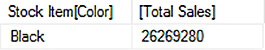
You can create more complex filter conditions by using OR or AND logic. Listing 3-56 shows two examples of using OR logic to filter the query results to include sales only when a stock item is Black or Blue. The first example uses the OR function which takes two arguments and returns TRUE when either argument is FALSE or FALSE when both arguments are FALSE. The second example uses the OR operator (||) to evaluate conditions on either side of the operator and applies the same logic used by the OR function to return either TRUE or FALSE. Both queries produce the same result shown in Figure 3-55.
Note Logical AND
Similarly, you have two choices when creating a filter condition for a logical AND. You can use the AND function, which returns TRUE only when both arguments are TRUE or FALSE when either argument is FALSE. As an alternative, you can use the AND operator (&&) to evaluate conditions on either side of the operator.
LISTING 3-56 FILTER function with OR logic
// Using the OR function
EVALUATE
SUMMARIZE(
FILTER(
'Sale',
OR(RELATED('Stock Item'[Color]) = "Black",
RELATED('Stock Item'[Color]) = "Blue"
)
),
'Stock Item'[Color],
"Total Sales",
'Sale'[Total Sales]
)
// Using the || operator
EVALUATE
SUMMARIZE(
FILTER(
'Sale',
RELATED('Stock Item'[Color]) = "Black" ||
RELATED('Stock Item'[Color]) = "Blue"
),
'Stock Item'[Color],
"Total Sales",
'Sale'[Total Sales]
)
Note Comments in DAX
You can include comments in a DAX query by preceding the comment with //. Comments can appear between lines of code or at the end of a line of code.

As an alternative to using the AND operator when you have multiple conditions to apply, you can nest FILTER functions, as shown in Listing 3-57. The result shown in Figure 3-56 is effectively the same result returned by using the AND operator. However, you might find that nesting FILTER functions perform better than using the AND operator, especially when the innermost filter returns a smaller result set than the outermost filter.
LISTING 3-57 Nested FILTER functions
EVALUATE
SUMMARIZE(
FILTER(
FILTER(
'Sale',
RELATED('Date'[Calendar Year Label]) = "CY2016"
),
RELATED('Stock Item'[Color]) = "Black"
),
'Stock Item'[Color],
"Total Sales",
'Sale'[Total Sales]
)
Besides filtering columns to display only rows matching a specific label, as shown in the previous examples, you can also filter columns based on a comparison of numeric values. Furthermore, you can apply filters to data that has been aggregated. Let’s say that you want to display a list of cities and total sales for each city, but you also want to filter this list to include only cities for which sales exceed 400,000. To do this, you must break down the query into two steps. Your first step is to produce a summarized table of cities and then you can apply a filter to the summarized table as your second step, as shown in Listing 3-58. The query resolves the innermost function first to produce a table containing aggregated sales by city, and then applies the filter to this table.
LISTING 3-58 Filter by measure
EVALUATE
FILTER(
SUMMARIZE(
'Sale',
'City'[City Key],
'City'[City],
"Total Sales",
'Sale'[Total Sales]
),
[Total Sales] > 400000
)
ORDER BY
'City'[City]
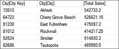
ALL function
Whether a filter is applied to query results explicitly by the FILTER function or implicitly by an expression’s filter context, DAX provides functions to selectively remove or retain current filters. One way to do this is to use the ALL function as described in the “CALCULATE function” section earlier in this chapter. In that example, the argument for the ALL function is a table, but you can also use columns as arguments for the ALL function.
Let’s revisit the example used to introduce the CALCULATE function in which the query produces a percentage of total sale count by sales territory. This time, you want to modify the query to show the percentage break down for each year by sales territory. In other words, for each year, the query should return the relative contribution of each sales territory, as you can see in the partial query results shown in Figure 3-58. That means you need to remove the filter for sales territory in the denominator only and retain the filter for year. That way, the denominator includes sales for all territories for the current year. To do this, use the ALL function with the column reference to the Sales Territory in the City table, as shown in Listing 3-59.
LISTING 3-59 ALL function to remove filter on a specific column
DEFINE
MEASURE 'Sale'[Overall Sale Count] =
CALCULATE(
COUNTROWS('Sale'),
ALL('City'[Sales Territory])
)
MEASURE 'Sale'[Percent of Total Sale Count] =
'Sale'[Sale Count] / 'Sale'[Overall Sale Count]
EVALUATE
ADDCOLUMNS(
SUMMARIZE(
'Sale',
'Date'[Calendar Year Label],
'City'[Sales Territory],
"Sale Count",
'Sale'[Sale Count]
),
"Overall Sale Count",
'Sale'[Overall Sale Count],
"Percent of Total Sale Count",
'Sale'[Percent of Total Sale Count]
)
ORDER BY
'Date'[Calendar Year Label],
'City'[Sales Territory]

One of the limitations of using the ADDCOLUMNS function with a nested SUMMARIZE function in a query is the inability to also use the ROLLUP syntax to obtain subtotals for specified groups. However, you can use SUMMARIZE again as the outermost function as shown in Listing 3-60, and thereby produce the subtotals as you can see in the partial query results shown in Figure 3-59.
LISTING 3-60 Outer SUMMARIZE function with ROLLUP
DEFINE
MEASURE 'Sale'[Overall Sale Count] =
CALCULATE(
COUNTROWS('Sale'),
ALL('City'[Sales Territory])
)
MEASURE 'Sale'[Percent of Total Sale Count] =
'Sale'[Sale Count] / 'Sale'[Overall Sale Count]
EVALUATE
SUMMARIZE(
ADDCOLUMNS(
SUMMARIZE(
'Sale',
'Date'[Calendar Year Label],
'City'[Sales Territory],
"Sale Count",
'Sale'[Sale Count]
),
"Overall Sale Count",
'Sale'[Overall Sale Count],
"Percent of Total Sale Count",
'Sale'[Percent of Total Sale Count]
),
'Date'[Calendar Year Label],
ROLLUP('City'[Sales Territory]),
"Sale Count",
'Sale'[Sale Count],
"Overall Sale Count",
'Sale'[Overall Sale Count],
"Percent of Total Sale Count",
'Sale'[Percent of Total Sale Count]
)
ORDER BY
'Date'[Calendar Year Label],
'City'[Sales Territory]

ADDMISSINGITEMS function
When a query has no value for a combination of items from separate columns, the query results are filtered to exclude that combination. However, sometimes it is important to know that a particular combination does not exist. To override that filter and reveal those missing combinations, use the ADDMISSINGITEMS function, which is one of the new DAX functions in SQL Server 2016. The results of executing the two queries in Listing 3-61 are shown in Figure 3-60.
LISTING 3-61 ADDMISSINGITEMS function
// Missing combination of items is filtered from query results
EVALUATE
FILTER(
SUMMARIZE(
'Sale',
'City'[Sales Territory],
'Stock Item'[Color],
"Sale Count",
'Sale'[Sale Count]
),
'City'[Sales Territory] = "External"
)
ORDER BY
'City'[Sales Territory],
'Stock Item'[Color]
GO
// Missing combination of items is included in query results
EVALUATE
FILTER(
ADDMISSINGITEMS(
'City'[Sales Territory],
'Stock Item'[Color],
SUMMARIZE(
'Sale',
'City'[Sales Territory],
'Stock Item'[Color],
"Sale Count",
'Sale'[Sale Count]
),
'City'[Sales Territory],
'Stock Item'[Color]
),
'City'[Sales Territory] = "External"
)
ORDER BY
'City'[Sales Territory],
'Stock Item'[Color]

Note Additional syntax options for the ADDMISSINGITEMS function
You can use additional arguments to define rollup groups and apply a logical test to determine whether a value is a subtotal. For more information about these arguments and restrictions related to this function, see “ADDMISSINGITEMS Function (DAX)” at https://msdn.microsoft.com/en-us/library/dn802537.aspx.
ROW function
As you learned earlier in this chapter, you can produce combinations of items from different dimensions by creating tuple sets in MDX, but DAX works only with tables and columns. There is no set construct in DAX. However, you can simulate the effect of a tuple set by using the CALCULATE function with filters to set the items to combine together and then nest this function inside the ROW function to return a table containing a single row. Use the new UNION function to combine multiple tables. Figure 3-61 shows the results of executing the query shown in Listing 3-62.
LISTING 3-62 UNION and ROW functions
EVALUATE
UNION(
ROW(
"Stock Item",
"Black",
"Sales Territory",
"Southwest",
"Calendar Year",
"CY2016",
"Sales",
CALCULATE(
'Sale'[Total Sales],
'Stock Item'[Color] = "Black",
'City'[Sales Territory] = "Southwest",
'Date'[Calendar Year Label] = "CY2016",
'Customer'[Buying Group] = "Tailspin Toys",
'Stock Item'[Size] = "L"
)
),
ROW(
"Stock Item",
"Blue",
"Sales Territory",
"Far West",
"Calendar Year",
"CY2016",
"Sales",
CALCULATE(
'Sale'[Total Sales],
'Stock Item'[Color] = "Blue",
'City'[Sales Territory] = "Far West",
'Date'[Calendar Year Label] = "CY2016",
'Customer'[Buying Group] = "Tailspin Toys",
'Stock Item'[Size] = "L"
)
)
)

CALCULATETABLE function
The CALCULATETABLE function has the same behavior as the CALCULATE function, except that it returns a table whereas CALCULATE returns a scalar value. In many cases, you might find queries execute faster when you use the CALCULATETABLE to apply a filter to a table instead of the FILTER function. As an example, you can rewrite Listing 3-55 to instead use CALCULATETABLE, as shown in Listing 3-63, generating the same result.
LISTING 3-63 CALCULATETABLE function
EVALUATE
SUMMARIZE(
CALCULATETABLE(
'Sale',
'Stock Item'[Color] = "Black"
),
'Stock Item'[Color],
"Total Sales",
'Sale'[Total Sales]
)
Note CALCULATETABLE restrictions
There are some restrictions with which you should be familiar when using the CALCULATETABLE function. For example, the table expression in the first argument must be a function that returns a table. The second argument is either a table expression to use as a filter or a Boolean expression that cannot reference a measure, scan a table, or return a table. For more details, see “CALCULATETABLE Function (DAX)” at https://msdn.microsoft.com/en-us/library/ee634760.aspx.
Create calculated measures
As explained in Chapter 2, all measures in a tabular model are calculated and derived from an aggregation of values from multiple rows in a table. In that chapter, a few measures are added to the sample tabular model. You can create more complex measures in your tabular model by performing mathematical operations on aggregate values or manipulating filter and row context. Unlike calculated measures in multidimensional models in which aggregations are implied in the MDX expressions, you must explicitly specify an aggregate function in the DAX expression used for calculated measures in a tabular model. This section explores a variety of the more commonly used DAX functions to help you understand key concepts and function syntax, but does not provide complete coverage of all DAX functions. Links to additional information for the DAX functions are provided in the descriptions of each function category.
Exam Tip
SQL Server 2016 adds many new functions to the DAX language. You should be familiar with these new functions for which you can find a complete list at “New DAX Functions” at https://msdn.microsoft.com/en-us/library/mt704075.aspx. Some of these functions are more likely to be the subject of exam questions than others. Spend some time familiarizing yourself with functions in the following groups: date and time functions, information functions, filter functions, text functions, and other functions. In addition, practice using the new aggregate functions PRODUCT, PRODUCTX, MEDIAN, MEDIANX, and the group of percentile functions.
Mathematical functions
The majority of measures that you add to the model are likely to use basic mathematical operations and DAX functions. If you are familiar with Excel functions, many of the mathematical functions in DAX have similar names, syntax, and behavior, such as POWER and SQRT.
Note Mathematical and trigonometric functions
A complete list of mathematical and trigonometric functions in DAX is available at “Math and Trig Functions (DAX)” at https://msdn.microsoft.com/en-us/library/ee634241.aspx. Valid DAX operators at listed in “DAX Operator Reference” at https://msdn.microsoft.com/en-us/library/ee634237.aspx.
Aggregate functions
Because a measure returns a single value, the value that it returns is typically an aggregation of values. The most commonly used aggregate function is SUM, which was introduced in Chapter 2. Other common aggregation functions include AVERAGE, MIN, and MAX. Each of these aggregate functions takes a column, not an expression, as its only argument, returning a single value. The column must contain a numeric or date data type.
Remember that a measure’s value is subject to evaluation context in a query, as described earlier in this chapter. Similarly, rows, columns, filters, and slicers in a pivot table or Power View report apply a filter context to the measure and reduce the rows included in the aggregation of the measure’s value.
Another useful aggregate function is COUNTROWS, which differs from the other aggregate functions because its argument is a table instead of a column. It can also use an expression. As its name implies, it counts all the rows in a table, subject to filter context.
DAX also includes a special set of aggregate functions that allow you to use a column that contains both numeric and non-numeric text: AVERAGEA, MINA, MAXA, and COUNTA. Within this group, you might find COUNTA the most useful, because it returns the number of non-empty rows in a column.
The opposite approach of COUNTA for row counts is to use COUNTBLANK to count the number of empty rows in a column. Together, the combined results of COUNTA and COUNTBLANK is the same value as COUNTROWS.
Note DAX aggregate function list
You can find a list of DAX aggregate functions and links to the respective documentation at “Statistical Functions (DAX)” at https://msdn.microsoft.com/en-us/library/ee634822.aspx.
Iterator aggregate functions
Another special set of iterator aggregate functions have X as the suffix, such as SUMX introduced earlier in the “Evaluation context” section of this chapter. The first argument of this type of function is a table or table expression, and the second argument is an expression to evaluate. This group of functions differs from standard aggregate functions because they perform an aggregate operation on an expression rather than a column. More specifically, the expression is evaluated by using row context for each row in a table or a table expression and then the results from each row are produced by using the applicable aggregation function.
The functions in this group, such as AVERAGEX, MINX, and MAXX, behave like SUMX. The COUNTX function is slightly different in that it increments a count when the expression value is not blank. You can learn how these functions work by updating the sample tabular model in your 70-768-Ch2 solution to include the measures shown in Table 3-3.
Note Import SSAS tabular project
If you do not have the 70-768-Ch2 solution from Chapter 2, but have restored the 70-768-Ch2.ABF file from the sample code files to your SSAS server, you can create a project from the restored database in SSDT. Point to New on the File menu, click Project, select Import From Server (Tabular), type a name for the project and solution, specify a location for the solution, and click OK. Connect to your tabular server, and select the 70-768-Ch2 database. On the Model menu, point to Process, and then click Process All to load the workspace for your model with data.

The first argument in the City Sale Count measure, VALUES(‘City’[WWI City ID], creates a table of the distinct values in the WWI City ID column. That way, the duplicate rows in the table resulting from slowly changing dimension handling (described in Chapter 1), do not result in an overstatement of the number of cities like the City Count measure does. The COUNTX function iterates over this table of 656 rows, and then, for each city’s row, resolves the second argument, which gets the sum of total sales for that city. Remember that the row context of the City table applies as a filter context in the Sale table. If there is a non-blank value, the count value is incremented. You can think of this measure as a flag to indicate when any sales exist for a given city.
The City Sale over 15K Count measure is similar, but its goal is to flag a city whenever it has a sale over $15,000. The CALCULATE function in the second argument filters the Total Sales measure to aggregate rows for the city in the current row from the first argument where the Sale row’s Total Excluding Tax value exceeds 15,000. Note that this measure does not count how many sales are over 15,000 for a city, but only whether there are any sales over that amount.
To check the new measures, save the model, and then click Analyze In Excel, which opens a workbook containing a pivot table connected to your model. In the PivotTable Fields list, select the following check boxes: City Sale Count, City Sale Count over 1K, and State Province. A portion of the resulting pivot table is shown in Figure 3-62.

DIVIDE function
A common business requirement is to analyze ratios that require measures that use division. One way to do this is to use the division operator (/) to compute Profit Margin Percent, like this:
Profit Margin Percent := SUM(Sale[Profit]) / [Total Sales]
In this measure expression, the numerator applies the SUM aggregate function to the Profit column, but uses the Total Sales measure as the numerator without applying the SUM function. Because the Total Sales measure already applies the SUM function to the Total Excluding Tax column, the aggregate function is not required in the measure referencing it. While technically accurate, a problem with this measure expression is the potential for a divide-by-zero error. You can avoid this problem by enclosing the expression inside a logical expression (described later in this chapter in the “Logical functions” section) or by using the DIVIDE function, like this:
Profit Margin Percent := DIVIDE(SUM(Sale[Profit]) , [Total Sales] )
Date and time functions
Most DAX date and time functions are more useful for expressions in calculated columns than in measures. One new date function added to DAX in SQL Server 2016 Analysis Services, however, is DATEDIFF. When you have two dates that can be compared in the same row context, you can compute the difference between them. As an example, add the following measure to the tabular model configured as a Decimal Number with two decimal places:
Delivery Interval:=
AVERAGEX('Sale',
DATEDIF/F(
'Sale'[Invoice Date Key],
'Sale'[Delivery Date Key],
DAY)
)
In the Wide World Importers DW database, the difference between the two date columns is generally one day, so the Delivery Interval measure is not enlightening from an analytical point of view. If there was more variance, you could assess how delivery intervals trend over time by location or by customer, to name only two examples. Nonetheless, it does serve to illustrate how to structure a measure using the DATEDIFF function, which returns an integer that you can then use to compute an average in the Sale table. The first and second arguments of this function are the start date and end date, respectively. The third argument is the interval to use for date comparisons, which can be any of the following values: SECOND, MINUTE, HOUR, DAY, WEEK, MONTH, QUARTER, or YEAR.
Note DAX date and time function list
You can find a list of DAX date and time functions with links to more information at “Date and Time Functions (DAX)” at https://msdn.microsoft.com/en-us/library/ee634786.aspx.
Time intelligence functions
The ability to perform time series analysis is a common requirement for a business intelligence solution. DAX provides a wide variety of functions to support this requirement. In this section, you explore the usage of the following three functions: TOTALYTD, SAMEPERIODSLASTYEAR, and PREVIOUSMONTH. To get started, update the tabular model by adding and configuring the measures shown in Table 3-4.

After saving the model, check the results by setting a pivot table as shown in Figure 3-63 by selecting the following check boxes: Total Sales, Total Sales YTD, Previous Month Sales, Prior Year Sales, and Prior YTD Sales. Then drag the Calendar hierarchy to the Rows pane below the PivotTable Fields list to produce the pivot table shown in Figure 3-63. Let’s examine how each measure is evaluated:
![]() Total Sales YTD The TOTALYTD function takes a scalar value expression as its first argument, which in this case is the Total Sales measure. The second argument is a column containing a series of dates. To see a value returned for this measure, you must place items from the table containing the dates column on rows, columns, filters, or slicers in a pivot table, or include the item’s column in a query. This column from the date table sets the row context used to calculate a value in the query results.
Total Sales YTD The TOTALYTD function takes a scalar value expression as its first argument, which in this case is the Total Sales measure. The second argument is a column containing a series of dates. To see a value returned for this measure, you must place items from the table containing the dates column on rows, columns, filters, or slicers in a pivot table, or include the item’s column in a query. This column from the date table sets the row context used to calculate a value in the query results.
As an example, the value for CY2013-Feb sets the filter context and includes a range of dates from the beginning of the year, 2013-01-01, to the last date in February, 2013-02-28. The Total Sales value for each of these dates are summed to produce the value of 6,547,197.05.
![]() Previous Month Sales The PREVIOUSMONTH function is used as a filter in a CALCULATE function to manipulate the filter context on Total Sales. Note the use of the Date column from the Date table, a common pattern to use when working with time intelligence functions. Again, it sets the row context.
Previous Month Sales The PREVIOUSMONTH function is used as a filter in a CALCULATE function to manipulate the filter context on Total Sales. Note the use of the Date column from the Date table, a common pattern to use when working with time intelligence functions. Again, it sets the row context.
In the query results shown in Figure 3-63, the row context in row 4 is CY2013-Feb. This row context is used as a starting point to find the previous month, which is CY2013-Jan. That month is then used to filter the Total Sales value to 3,770,410.85, which is returned as Previous Month Sales on row 4.
![]() Prior Year Sales Conceptually, the formula for Prior Year Sales is similar to Previous Month Sales. This time the filter condition uses the SAMEPERIODLASTYEAR to set the row context based on the Date column.
Prior Year Sales Conceptually, the formula for Prior Year Sales is similar to Previous Month Sales. This time the filter condition uses the SAMEPERIODLASTYEAR to set the row context based on the Date column.
If you examine row 16, the row context for Date is CY2014-Jan. The SAMEPERIODLASTYEAR function navigates through dates to find the corresponding time period one year prior, which is CY2013-Jan. This date is used to filter Total Sales, to thereby return to 3,770,410.85. Likewise, row 15 uses the date context of CY2014. In that case, the SAMEPERIODLASTYEAR returns a new row context of CY2013, which has a Total Sales value of 45,707,188, to compute Prior Year Sales.
![]() Prior YTD Sales In this case, the SAMPERIODLASTYEAR function finds the corresponding time period to determine the current row’s corresponding date one year earlier. This time period is passed to the DATESYTD function to create a date range from the beginning of the year to the end date returned by SAMEPERIODLASTYEAR. Thus, the Prior YTD Sales for CY2014-Mar matches the Total Sales YTD for CY2013-Mar.
Prior YTD Sales In this case, the SAMPERIODLASTYEAR function finds the corresponding time period to determine the current row’s corresponding date one year earlier. This time period is passed to the DATESYTD function to create a date range from the beginning of the year to the end date returned by SAMEPERIODLASTYEAR. Thus, the Prior YTD Sales for CY2014-Mar matches the Total Sales YTD for CY2013-Mar.

Note DAX time intelligence function list
Refer to “Time Intelligence Functions (DAX)” at https://msdn.microsoft.com/en-us/library/ee634763.aspx to learn more about the available time intelligence functions.
Filter functions
Several different filter functions are described in the “Filter DAX queries” section earlier in this chapter. In those earlier examples, the emphasis is the use of filters to affect the rows returned in the query results. You can also use filter functions to reduce the items on which aggregate functions operate.
Let’s say you want to add enable analysis of sales for Tailspin Toys in conjunction with all sales. By setting up filtered measures, you can compare Tailspin Toys side by side with sales to all customers. Update your tabular model by adding the measures shown in Table 3-5, as described in Chapter 2.

Save the model, and then click Analyze In Excel. Create a pivot table using the following measures: Total Sales, Tailspin Toys Total Sales, and Tailspin Toys % Of Total Sales. Then place Sales Territory on rows to produce the pivot table shown in Figure 3-64. The creation of filtered measures allows you to focus on groups of interest, such as Tailspin Toys, individually and in comparison to all sales.

The complete list of filter functions available in DAX is available at “Filter Functions (DAX)” at https://msdn.microsoft.com/en-us/library/ee634807.aspx.
Logical functions
Logical functions either return a TRUE or FALSE value or evaluate conditions as TRUE or FALSE to determine which values to return. Among the group of logical functions are the IF and SWITCH functions. Also in this group are the AND and OR functions explained earlier in this chapter.
The IF function is useful for a simple condition and requires only two arguments. The first argument is a Boolean expression to evaluate, and the second argument is a value or expression returning a value if the Boolean expression is TRUE. Optionally, you can add a third argument to return a value for a FALSE condition. You can nest IF functions for more complex conditional scenarios.
The SWITCH argument is useful when you have several conditions to evaluate and is easier to read than a series of nested IF functions. As an example, add the following measure to your tabular model:
Sales Group:=
SWITCH(
TRUE(),
[Total Sales] < 1000000, "Under 1,000,000",
[Total Sales] < 10000000, "Between 1,000,000 - 10,000,000",
[Total Sales] < 2000000, "Between 10,000,000 - 20,000,000",
"Over 20,000,000"
)
Not only does the Sales Group measure illustrate how to use the SWITCH function, it also shows how a measure is not required to return a numeric value. You can use this technique to assign a label to groups based on specified criteria, as shown in Figure 3-65.

Note DAX logical function list
You can learn more about DAX logical functions by reviewing the list of available functions at “Logical Functions (DAX)” at https://msdn.microsoft.com/en-us/library/ee634365.aspx.
Variables
In SQL Server 2016, you can use variables in a DAX expression to make it easier to understand the logic in a complex expression. Variables are flexible in that you can use them to store any type of object, such as a column, a table, or a value. Additionally, the use of a variable can potentially improve query performance when the same logic is used repeatedly in the same expression, because the variable is evaluated only once. However, a variable has scope only within the measure in which you define it.
Table 3-6 is a set of measures to add to the Sale table in your tabular model to illustrate the use of variables. These measures are a variation on the theme of filtering measures to focus on a specific group. Notice the use of VAR to prefix the variable name, and then RETURN to mark the beginning of the expression to resolve to a scalar value.
Note Formula bar expansion
Click the arrow on the right side of the bar to expand the window so that you can more easily work with expressions containing multiple lines.


Figure 3-66 shows the results of these new measures added to a pivot table with Sales Territory on rows. The Internal All Sales and Internal Sales Over 15K measures exist in this example solely to allow you to validate the results of the Internal > $15K % of Total Sales measure. Let’s take a closer look at how the Internal > $15K % of Total Sales measure is evaluated by using the following three variables:
![]() InternalTerritories A table of Sales Territories that is filtered to exclude the External and N/A sales territories. In other words, it includes the Internal sales territories.
InternalTerritories A table of Sales Territories that is filtered to exclude the External and N/A sales territories. In other words, it includes the Internal sales territories.
![]() InternalSalesOver15K A scalar value derived by iterating over the InternalTerritories table, which is filtered to a subset of rows for which Total Excluding Tax is greater than 15000 and then the Total Sales value for these rows is summed. The result is a measure that reflects the total sales for any sales territory if any of its sales exceed 15,000.
InternalSalesOver15K A scalar value derived by iterating over the InternalTerritories table, which is filtered to a subset of rows for which Total Excluding Tax is greater than 15000 and then the Total Sales value for these rows is summed. The result is a measure that reflects the total sales for any sales territory if any of its sales exceed 15,000.
![]() InternalAllSales A scalar value derived by iterating over the unfiltered InternalTerritories table to sum the Total Sales value for all rows. This measure represents an overall value to be used later to compute a ratio.
InternalAllSales A scalar value derived by iterating over the unfiltered InternalTerritories table to sum the Total Sales value for all rows. This measure represents an overall value to be used later to compute a ratio.
The formula that returns a value for this measure uses the DIVIDE function to derive the ratio between InternalSalesOver15K and InternalAllSales. The use of variables in this formula makes it easier to understand the logic as compared to nesting the functions and expanding the logic inside the DIVIDE function.

Note Variables
You can define variables inside expressions rather than define them at the beginning of the measure code. Alberto Ferrari describes variable syntax options in his article “Variables in DAX,” which you can read at https://www.sqlbi.com/articles/variables-in-dax/.
Perform analysis by using DAX
There are many different types of analysis that you can perform by using DAX to create expressions for measures and calculated columns in your tabular model. Just as this chapter cannot cover every possible DAX function, this section cannot provide guidance for every possible type of analysis that you might need to perform in real-world applications. However, it should provide some insight into additional ways that you can use DAX.
Top ranked items
When you need to find items in a column having the highest measure values or highest ranking, you can use the TOPN function in a query. The first argument in this function is the number of items to return, and the second argument is a table expression to evaluate. In Listing 3-64, the table expression is a summary table that contains Total Sales for each stock item. The TOPN function sorts this column of stock items in the descending order of sales and returns the first five items, as shown in Figure 3-67.
EVALUATE
TOPN(
5,
SUMMARIZE(
'Stock Item',
'Stock Item'[Stock Item],
"Sales",
[Total Sales]
),
[Sales]
)

However, if the primary client tool for analyzing top items is Excel, it is easier to use the RANK function in a measure. Use the code in Listing 3-65 to add the following measure to the tabular model. In this case, the RANKX function behaves like other iterator aggregate functions. Its first argument is an unfiltered Stock Item table for which a rank for each item is determined based on Total Sales. The IF function then evaluates the rank assignment and returns the Total Sales value only if an individual stock item has a rank of 5 or lower. If a stock item has a different value, the function returns a blank value. You can then use Excel’s default behavior to ignore rows with a blank value when you use this measure in isolation and in a pivot table, as shown in Figure 3-68.
Top 5 Stock Items:=
VAR
SalesRank =
RANKX( ALL('Stock Item'), [Total Sales])
RETURN
IF(
SalesRank<=5,
[Total Sales]
)

Variance
Recall the example in Listing 3-54, which illustrated the impact that row context has on measure evaluation. The business requirement in that scenario is to calculate the number of sales in which a stock item color sells at some value below the average recommended retail price for all stock items sharing the same color. Put another way, the goal is to determine variance between one value and a stated baseline. Variance can be expressed both as a value representing the difference, or as a ratio comparing this difference to a target value. Let’s expand on the initial example to find the variance percentage between the average selling price and a baseline, which is the average recommended retail price for all stock items in a color group.
Table 3-7 is a set of measures to add to the Sale table in your tabular model to illustrate the use of DAX to calculate a variance percentage. Color Avg Retail $ finds the average retail price for all stock items in a color group, regardless of whether the item has sale transactions. The Avg Selling $ is the average price for which stock items have sold. The difference between these two values is computed and then divided by the baseline to return the variance percentage as Selling Variance %.

Figure 3-69 shows the results of adding these measures to the tabular model. You can see that the relative difference between selling price and recommended retail price changes by color group, with Yellow stock items having the smallest variance.
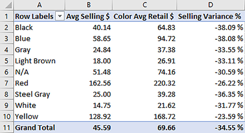
Ratio to parent
The use of CALCULATE to derive a percent of total was introduced in Listing 3-53. In that case, a row’s value is compared to an overall value in which all filters are removed. Listing 3-54 illustrated how to selectively remove filters to calculate an overall value for a subset of a table while retaining some of the row context for the active row. Now, let’s examine how to approach a ratio to percent calculation in which hierarchical relationships are considered. Strictly speaking, DAX does not understand how to navigate hierarchies in the same way that you use navigation functions in MDX to traverse user-defined hierarchies. Nonetheless, you can construct expressions to achieve the same results.
Table 3-8 is a set of measures to add to the Sale table in your tabular model to illustrate the construction of ratio to parent calculations. In these examples, the hierarchy is the Calendar hierarchy for dates, months, and years, but you can use the same technique in any table for which you have created a multi-level hierarchy.


As you can see in Figure 3-70, the Ratio to Month measure returns a ratio that compares a current date’s value to all dates within the month. In this case, the filter on each row removes only the date filter, but retains the month and year filters. Then the ISFILTERED function determines whether to return a value. On row 4, the Ratio To Month value is computed by dividing the Total Sales value of 28,475.10, filtered for 1/1/2013, by the value for Total Sales that is not filtered by date. However, the month filter still applies to the divisor in the Ratio To Month expression. In this case, the month filter is CY2013-Jan, which means the divisor in the expression on row 4 is the 3,770,410.85. Thus, the division of 28,475.10 by 3,770,410.85 results in the Ratio To Month value of 0.76%.

The other measures work similarly for the respective levels, but introduce NOT ISFILTERED to reverse the logical condition used to determine whether a value is displayed. In effect, to return a value for Ratio To Year, the current month must have a month filter applied, but cannot have a date filtered applied also, as is the case on row 3 for which a Total Sales value for CY2013-Jan displays. This combination of conditions means that 3,770,410.85 represents a month total and not a day total. Therefore, SSAS can resolve the Ratio To Year value correctly by dividing this month value by the corresponding Total Sales value for the year (shown in row 2).
You can consolidate the code into a single measure by adding the measure shown in Listing 3-66 and formatting it as a percentage value. Because it uses nested IF functions, there is no longer a need to use the NOT ISFILTERED pattern. When the expression evaluation moves to the code related to months, for example, the determination was made in the outer IF function that the active row is not a date. Thus, this expression simplifies the code in the previous examples. You can see the results of the new expression in Figure 3-71. Although this single expression is simpler, you may find it more challenging to troubleshoot. In that case, you can create separate measures and use the Hide From Client Tools option to prevent users from accessing these intermediate measures directly.
LISTING 3-66 Ratio to parent expression
Ratio To Parent:=
VAR
SalesAllDates =
CALCULATE(
[Total Sales],
ALL('Date'[Date])
)
VAR
SalesAllMonths =
CALCULATE(
[Total Sales],
ALL('Date'[Calendar Month Label])
)
VAR
SalesAllYears =
CALCULATE(
[Total Sales],
ALL('Date'[Calendar Year Label])
)
RETURN
IF(
ISFILTERED('Date'[Date]) ,
DIVIDE(
[Total Sales] ,
SalesAllDates
),
IF(
ISFILTERED('Date'[Calendar Month Label] ) ,
DIVIDE(
[Total Sales] ,
SalesAllMonths
),
IF(
ISFILTERED('Date'[Calendar Year Label]) ,
DIVIDE(
[Total Sales] ,
SalesAllYears
),
1
)
)
)

Note Slicing with hierarchy items yields incorrect results
If you add a slicer to the worksheet and attempt to slice by an item that also appears in the hierarchy in the pivot table, the ratio to parent calculation no longer works correctly. Alberto Ferrari suggests a solution to this problem in his article, “Clever Hierarchy Handling in DAX,” at http://www.sqlbi.com/articles/clever-hierarchy-handling-in-dax/.
Allocation
The “Define a SCOPE statement” section in Skill 3.2 introduced business requirements for sales quota allocations for which you can create calculations in the MDX script that give the illusion of inserting values into cells to replace existing values or add values where none existed. Although a tabular model does not have an MDX script, you can achieve a similar technique by adapting the technique described in the “Ratio to parent” section.
Before you can create the measures necessary for the allocations, add a new calculated column to the Date table by using the following expression:
=DAY(EOMONTH([Date],0))
The EOMONTH function uses the active row context to find the last day of the current day’s month. Then the DAY function returns the month number associated with that date. This number conveniently represents the number of days in a month that you can use to perform the sales quota allocations.
Listing 3-67 is a single measure expression that uses variables to make it easier to follow the logic in the code that relies on a combination of IF and SWITCH function to determine what calculation to perform for each level in the calendar hierarchy. Let’s review the following key elements of this code:
![]() The quota for 2014 is a hardcoded value stored in the Quota2014Month variable.
The quota for 2014 is a hardcoded value stored in the Quota2014Month variable.
![]() The 2015 quota is calculated according to the business requirements by multiplying the previous year’s sales by 110% and dividing by 12 to determine the monthly allocation. Notice the ALL function in that calculation removes both month and date level filers to ensure the calculation is correct on either level. (Try removing it to observe the effect.)
The 2015 quota is calculated according to the business requirements by multiplying the previous year’s sales by 110% and dividing by 12 to determine the monthly allocation. Notice the ALL function in that calculation removes both month and date level filers to ensure the calculation is correct on either level. (Try removing it to observe the effect.)
![]() The DaysInMonth variable calculates the number of days in the current context based on the MonthDays calculated column.
The DaysInMonth variable calculates the number of days in the current context based on the MonthDays calculated column.
![]() The Quota2014Days and Quota2015Days calculations divide the respective monthly quota by the number of days in the current month.
The Quota2014Days and Quota2015Days calculations divide the respective monthly quota by the number of days in the current month.
![]() Each level of the hierarchy is represented in nested IF functions, starting with Date in the outermost IF function and ending with Calendar Year Label in the innermost function. The IF function uses ISFILTERED to test whether the current item is a date, month, or year.
Each level of the hierarchy is represented in nested IF functions, starting with Date in the outermost IF function and ending with Calendar Year Label in the innermost function. The IF function uses ISFILTERED to test whether the current item is a date, month, or year.
![]() When an IF function evaluates as TRUE, the corresponding SWITCH statement is evaluated. The SWITCH statement evaluates a table of values for the current row to determine whether it relates to CY2014 or CY2015 and then returns the daily quota on the date level and, the month quota on the month level, as you can see in Figure 3-72. On the year level, the appropriate month quota is multiplied by 12, as you can see in Figure 3-73.
When an IF function evaluates as TRUE, the corresponding SWITCH statement is evaluated. The SWITCH statement evaluates a table of values for the current row to determine whether it relates to CY2014 or CY2015 and then returns the daily quota on the date level and, the month quota on the month level, as you can see in Figure 3-72. On the year level, the appropriate month quota is multiplied by 12, as you can see in Figure 3-73.
LISTING 3-67 Allocation expression
Sales Quota:=
VAR
Quota2014Month = 4500000
VAR
Quota2015Month =
DIVIDE(
CALCULATE(
[Prior Year Sales] *1.1,
ALL('Date'[Calendar Month Label],
'Date'[Date])
),
12
)
VAR
DaysInMonth =
SUMX( 'Date',
CALCULATE(
VALUES( 'Date'[MonthDays])
)
)
VAR
Quota2014Days =
DIVIDE(
Quota2014Month,
DaysInMonth
)
VAR
Quota2015Days =
DIVIDE(
Quota2015Month,
DaysInMonth
)
RETURN
IF(
ISFILTERED('Date'[Date]),
SWITCH(
VALUES('Date'[Calendar Year Label]),
"CY2014", Quota2014Days,
"CY2015", Quota2015Days
) ,
IF (
ISFILTERED('Date'[Calendar Month Label]) ,
SWITCH(
VALUES('Date'[Calendar Year Label]),
"CY2014", Quota2014Month,
"CY2015", Quota2015Month
),
IF (
ISFILTERED('Date'[Calendar Year Label]),
SWITCH(
VALUES('Date'[Calendar Year Label]),
"CY2014", Quota2014Month * 12,
"CY2015", Quota2015Month * 12
)
)
)
)


Need More Review? DAX for analysis
You can find a variety of use cases and DAX patterns for analysis developed by Marco Russo and Alberto Ferrari on their DAX Patterns site at http://daxpatterns.com.
Chapter summary
![]() The basic structure of an MDX query looks like this:
The basic structure of an MDX query looks like this:
WITH
MEMBER <Name> AS <definition>
SET <Name> AS <definition>
SELECT
<Set> ON COLUMNS,
<Set> ON ROWS
FROM
<Cube>
WHERE
<Tuple>;
![]() Although an MDX query’s structure is similar to the structure of a T-SQL query, its behavior is quite different. The sets that you define in the SELECT clause by placing them on rows or columns are processed as the first steps of query processing. This evaluation of axes occurs independently of subsequent steps. Each cell intersection of set members on rows and columns defines a partial tuple that is combined with members included in the query’s WHERE clause and the default member of every attribute hierarchy that is not explicitly defined in the query to produce a full tuple. This full tuple represents a cube cell value that is returned in the query results. A tuple is a coordinate in multidimensional space.
Although an MDX query’s structure is similar to the structure of a T-SQL query, its behavior is quite different. The sets that you define in the SELECT clause by placing them on rows or columns are processed as the first steps of query processing. This evaluation of axes occurs independently of subsequent steps. Each cell intersection of set members on rows and columns defines a partial tuple that is combined with members included in the query’s WHERE clause and the default member of every attribute hierarchy that is not explicitly defined in the query to produce a full tuple. This full tuple represents a cube cell value that is returned in the query results. A tuple is a coordinate in multidimensional space.
![]() You place sets on the rows and columns of a query axis. A set can be empty or contain one or more members of the same dimension’s attribute hierarchy or user-defined hierarchy. You enclose a set within braces, although you can omit the braces when a set contains a single member.
You place sets on the rows and columns of a query axis. A set can be empty or contain one or more members of the same dimension’s attribute hierarchy or user-defined hierarchy. You enclose a set within braces, although you can omit the braces when a set contains a single member.
![]() You place tuples in the WHERE clause of a query. A tuple consists of one or more members of different attribute or user-defined hierarchies. You can create sets of tuples to place on axes in the SELECT clause.
You place tuples in the WHERE clause of a query. A tuple consists of one or more members of different attribute or user-defined hierarchies. You can create sets of tuples to place on axes in the SELECT clause.
![]() Tuples and sets can be explicitly defined by referencing members by name or by unique name or you can use functions that return members and sets.
Tuples and sets can be explicitly defined by referencing members by name or by unique name or you can use functions that return members and sets.
![]() MDX functions use one of the following syntax patterns:
MDX functions use one of the following syntax patterns:
![]() The argument pattern places the function first in an expression which is followed by one or more arguments enclosed in parentheses, like this: ORDER(<set>, <numeric or string expression>, <sort direction>).
The argument pattern places the function first in an expression which is followed by one or more arguments enclosed in parentheses, like this: ORDER(<set>, <numeric or string expression>, <sort direction>).
![]() The method pattern places the function last in an expression by appending it to the end of an object, like this: [Dimension].[Hierarchy].[Member].Members.
The method pattern places the function last in an expression by appending it to the end of an object, like this: [Dimension].[Hierarchy].[Member].Members.
![]() When learning a new MDX function, you should understand what type of object it operates on or takes as an argument, such as a set or a member, and what type of object it returns, such as a tuple or a set.
When learning a new MDX function, you should understand what type of object it operates on or takes as an argument, such as a set or a member, and what type of object it returns, such as a tuple or a set.
![]() You should be familiar with the more commonly used MDX functions which are grouped into the following categories:
You should be familiar with the more commonly used MDX functions which are grouped into the following categories:
![]() Set functions Returns a set. Functions in this group include: MEMBERS, ORDER, HEAD, TOPCOUNT, NONEMPTY, FILTER, and DESCENDANTS.
Set functions Returns a set. Functions in this group include: MEMBERS, ORDER, HEAD, TOPCOUNT, NONEMPTY, FILTER, and DESCENDANTS.
![]() Navigation functions Returns a member when navigating to a higher level or a set when navigating to a lower level. Navigation on the same level can return a member or a set. Functions in this group include: PARENT, CHILDREN, ANCESTOR, SIBLINGS, PREVMEMBER, and NEXTMEMBER.
Navigation functions Returns a member when navigating to a higher level or a set when navigating to a lower level. Navigation on the same level can return a member or a set. Functions in this group include: PARENT, CHILDREN, ANCESTOR, SIBLINGS, PREVMEMBER, and NEXTMEMBER.
![]() Time functions Returns a member of a set. Functions in this group include: OPENING PERIOD, CLOSINGPERIOD, PARALLELPERIOD, and PERIODSTODATE.
Time functions Returns a member of a set. Functions in this group include: OPENING PERIOD, CLOSINGPERIOD, PARALLELPERIOD, and PERIODSTODATE.
![]() Statistical functions Returns a calculated value. Functions in this group include: SUM, and AGGREGATE,
Statistical functions Returns a calculated value. Functions in this group include: SUM, and AGGREGATE,
![]() String functions Returns a string or converts a string into an object such as a member or a set. Functions in this group include: SETTOSTR, STRTOMEMBER, NAME, UNIQUENAME, and PROPERTIES.
String functions Returns a string or converts a string into an object such as a member or a set. Functions in this group include: SETTOSTR, STRTOMEMBER, NAME, UNIQUENAME, and PROPERTIES.
![]() Use the NON EMPTY keyword to eliminate a row or a column when all of its related tuples are empty. This elimination is the last step of query processing.
Use the NON EMPTY keyword to eliminate a row or a column when all of its related tuples are empty. This elimination is the last step of query processing.
![]() Query-scoped calculations allow you to create calculated members, calculated measures, or sets that can be referenced within a query, but are not persisted to the cube. They are useful for ad hoc reporting and for testing logic before implementing it as a cube object.
Query-scoped calculations allow you to create calculated members, calculated measures, or sets that can be referenced within a query, but are not persisted to the cube. They are useful for ad hoc reporting and for testing logic before implementing it as a cube object.
![]() You can embed business logic into a cube by using custom MDX to create the following objects:
You can embed business logic into a cube by using custom MDX to create the following objects:
![]() Calculated measures Calculations that are assigned to the Measures dimension that you can reference in a tuple.
Calculated measures Calculations that are assigned to the Measures dimension that you can reference in a tuple.
![]() Calculated members Calculations that are assigned to a non-measure dimension that you can reference in sets.
Calculated members Calculations that are assigned to a non-measure dimension that you can reference in sets.
![]() Named sets Calculations that are assigned to a non-measure dimension and return a set. Members of a dynamic named set can change based on query context, whereas member of a static named set remain fixed regardless of query context.
Named sets Calculations that are assigned to a non-measure dimension and return a set. Members of a dynamic named set can change based on query context, whereas member of a static named set remain fixed regardless of query context.
![]() Statistical functions Returns a calculated value. Functions in this group include SUM and AGGREGATE.
Statistical functions Returns a calculated value. Functions in this group include SUM and AGGREGATE.
![]() String functions Returns a string or converts a string into an object such as a member or a set. Functions in this group include: SETTOSTR, STRTOMEMBER, NAME, UNIQUENAME, PROPERTIES.
String functions Returns a string or converts a string into an object such as a member or a set. Functions in this group include: SETTOSTR, STRTOMEMBER, NAME, UNIQUENAME, PROPERTIES.
![]() Every attribute hierarchy as an implicit default member, which is the All member on the top level of the hierarchy. You can define an explicit default member in the attribute’s properties or in role-based security configuration.
Every attribute hierarchy as an implicit default member, which is the All member on the top level of the hierarchy. You can define an explicit default member in the attribute’s properties or in role-based security configuration.
![]() You can use MDX to define allowed or denied sets for each dimension’s attributes or to set cell-level security to control the visibility of measures and calculated measures.
You can use MDX to define allowed or denied sets for each dimension’s attributes or to set cell-level security to control the visibility of measures and calculated measures.
![]() You can create your own MDX functions by developing and registering an Analysis Services Stored Procedure.
You can create your own MDX functions by developing and registering an Analysis Services Stored Procedure.
![]() Use a SCOPE statement in a cube’s MDX script to override cube cell values in a targeted section of the cube known as a subcube.
Use a SCOPE statement in a cube’s MDX script to override cube cell values in a targeted section of the cube known as a subcube.
![]() The basic structure of a DAX query looks like this:
The basic structure of a DAX query looks like this:
DEFINE
MEASURE <Name> = <expression>
EVALUATE
<table expression>
ORDER BY
<column> <sort direction>
![]() Commonly used functions in a query’s table expression are SUMMARIZE and ADDCOLUMNS.
Commonly used functions in a query’s table expression are SUMMARIZE and ADDCOLUMNS.
![]() An understanding of evaluation context is crucial to returning correct query results and developing measures. Filter context determines which rows in a table or column are subject to an operation and row context determines which columns are in scope for an operation.
An understanding of evaluation context is crucial to returning correct query results and developing measures. Filter context determines which rows in a table or column are subject to an operation and row context determines which columns are in scope for an operation.
![]() The CALCULATE function allows you to override filter context by removing filters completely or partially or by adding new filters. It also allows you to manipulate row context by projecting it as a filter context during table operations.
The CALCULATE function allows you to override filter context by removing filters completely or partially or by adding new filters. It also allows you to manipulate row context by projecting it as a filter context during table operations.
![]() A variety of DAX functions are available for creating calculated measures. You should be familiar with commonly used DAX functions in the following categories:
A variety of DAX functions are available for creating calculated measures. You should be familiar with commonly used DAX functions in the following categories:
![]() Aggregate functions Returns an aggregation of values based on a single column. Functions in this group include: SUM, AVERAGE, MIN, MAX, COUNTROWS, AVERAGEA, MINA, MAXA, COUNTA, and COUNTBLANK.
Aggregate functions Returns an aggregation of values based on a single column. Functions in this group include: SUM, AVERAGE, MIN, MAX, COUNTROWS, AVERAGEA, MINA, MAXA, COUNTA, and COUNTBLANK.
![]() Iterator aggregate functions Returns a value after iterating through rows of a table or table expression, resolving an expression for each row, and aggregating the results. Functions in this group include: SUMX, AVERAGEX, MINX, MAXX, and COUNTX.
Iterator aggregate functions Returns a value after iterating through rows of a table or table expression, resolving an expression for each row, and aggregating the results. Functions in this group include: SUMX, AVERAGEX, MINX, MAXX, and COUNTX.
![]() Date and time functions Return value depends on the function. Most functions in this category are used more often in calculated columns. For a measure, you can use the DATEDIFF function to calculate intervals between values in separate date columns.
Date and time functions Return value depends on the function. Most functions in this category are used more often in calculated columns. For a measure, you can use the DATEDIFF function to calculate intervals between values in separate date columns.
![]() Time intelligence functions Returns a date or date range that is used in turn to compute values. Functions in this group include: TOTALYTD, DATESYTD, SAMEPERIODLASTYEAR, PREVIOUSMONTH, DAY, and EOMONTH.
Time intelligence functions Returns a date or date range that is used in turn to compute values. Functions in this group include: TOTALYTD, DATESYTD, SAMEPERIODLASTYEAR, PREVIOUSMONTH, DAY, and EOMONTH.
![]() Filter functions Manipulates or evaluates filter context on a table. Functions in this group include: FILTER, ADDMISSINGITEMS, CALCULATE, CALCULATETABLE, ALL, ALLEXCEPT, ISFILTERED, RELATED, and VALUES.
Filter functions Manipulates or evaluates filter context on a table. Functions in this group include: FILTER, ADDMISSINGITEMS, CALCULATE, CALCULATETABLE, ALL, ALLEXCEPT, ISFILTERED, RELATED, and VALUES.
![]() Logical functions Returns information about values or expressions. Functions in this group include: IF, SWITCH, AND, and OR.
Logical functions Returns information about values or expressions. Functions in this group include: IF, SWITCH, AND, and OR.
![]() You can use variables to make complex DAX expressions easier to read and sometimes to improve performance by replacing multiple references to the same expression with a single variable which is evaluated once.
You can use variables to make complex DAX expressions easier to read and sometimes to improve performance by replacing multiple references to the same expression with a single variable which is evaluated once.
![]() Business analysis often focuses on comparisons of data points. You should be familiar with creating measures to create the following types of analysis:
Business analysis often focuses on comparisons of data points. You should be familiar with creating measures to create the following types of analysis:
![]() Top ranked items You can use TOPN in a query to return a group of ranked items, but use RANKX in a measure.
Top ranked items You can use TOPN in a query to return a group of ranked items, but use RANKX in a measure.
![]() Variance You can set up multiple measures that represent various perspectives of a calculation, such as all items in a table versus a filtered set of items or values at one point in time versus another point in time, and then compute the difference between those values. The CALCULATE function is frequently used in expressions that return a filtered value.
Variance You can set up multiple measures that represent various perspectives of a calculation, such as all items in a table versus a filtered set of items or values at one point in time versus another point in time, and then compute the difference between those values. The CALCULATE function is frequently used in expressions that return a filtered value.
![]() Ratio to parent When calculating ratios, you can use the CALCULATE function to remove filters on the current row to enable calculation of totals for its parent item and use the ISFILTERED function to determine whether to calculate a ratio and which values to use in the ratio calculation.
Ratio to parent When calculating ratios, you can use the CALCULATE function to remove filters on the current row to enable calculation of totals for its parent item and use the ISFILTERED function to determine whether to calculate a ratio and which values to use in the ratio calculation.
![]() Allocation Like the ratio to parent pattern, you can use the ISFILTERED function to determine whether a calculation should be performed. You can also use the SWITCH function to determine the type of calculation to perform.
Allocation Like the ratio to parent pattern, you can use the ISFILTERED function to determine whether a calculation should be performed. You can also use the SWITCH function to determine the type of calculation to perform.
Thought experiment
In this thought experiment, demonstrate your skills and knowledge of the topics covered in this chapter. You can find answer to this thought experiment in the next section.
You are the BI developer at Wide World Importers responsible for adding frequently used calculations to the multidimensional and tabular models referenced in this chapter and for responding to specific questions from users by creating ad hoc MDX or DAX queries. The following requirements have been identified:
![]() In the multidimensional model, you need to perform the following tasks:
In the multidimensional model, you need to perform the following tasks:
![]() Prepare a report that lists the top five stock items based on sales, total sales, and their respective rank.
Prepare a report that lists the top five stock items based on sales, total sales, and their respective rank.
![]() Update the cube so that users can easily add the top five stock items for any year to a pivot table. They must be able to apply filters to the pivot table to find the top stock items under different conditions.
Update the cube so that users can easily add the top five stock items for any year to a pivot table. They must be able to apply filters to the pivot table to find the top stock items under different conditions.
![]() Add annual quota allocations to the MDX script.
Add annual quota allocations to the MDX script.
![]() In the tabular model, you need to perform the following tasks:
In the tabular model, you need to perform the following tasks:
![]() The City Count measure currently counts the rows in the City table, but this overstates the true city count because there are duplicate rows in the table for many cities. Correct the City Count measure to return the correct number of cities.
The City Count measure currently counts the rows in the City table, but this overstates the true city count because there are duplicate rows in the table for many cities. Correct the City Count measure to return the correct number of cities.
![]() Update the tabular model to include a YTD Variance % calculation.
Update the tabular model to include a YTD Variance % calculation.
![]() Prepare a report that lists stock items and profit margin percent values for which the stock item’s aggregate profit margin percent is below 20 % in descending order of profitability.
Prepare a report that lists stock items and profit margin percent values for which the stock item’s aggregate profit margin percent is below 20 % in descending order of profitability.
Based on this background information, answer the following questions:
1. Which of the following MDX queries produces the ranked stock items report?
WITH
SET Top5Item AS
TOPCOUNT(
[Stock Item].[Stock Item].[Stock Item].Members,
5,
[Measures].[Sale Count]
)
MEMBER [Measures].[Rank] AS
RANK( [Stock Item].[Stock Item].CURRENTMEMBER, Top5Item)
SELECT
{[Measures].[Sales Amount Without Tax], [Measures].[Rank]} ON COLUMNS,
Top5Item ON ROWS
FROM [Wide World Importers DW]
LISTING B
WITH
SET Top5Item AS
TOPCOUNT(
[Stock Item].[Stock Item].Members,
5,
[Measures].[Sale Count]
)
MEMBER [Measures].[Rank] AS
ORDER( [Stock Item].[Stock Item].CURRENTMEMBER, [Measures].[Sale Count], DESC)
SELECT
{[Measures].[Sales Amount Without Tax], [Measures].[Rank]} ON COLUMNS,
Top5Item ON ROWS
FROM [Wide World Importers DW]
LISTING C
WITH
SET Top5Item AS
TOPCOUNT(
[Stock Item].[Stock Item].[Stock Item].Members,
5,
[Measures].[Sale Count]
)
MEMBER [Measures].[Rank] AS
RANK( [Stock Item].[Stock Item].CURRENTMEMBER, Top5Item)
SELECT
{[Measures].[Sales Amount Without Tax], [Measures].[Rank]} ON COLUMNS,
Top5Item ON ROWS
FROM [Wide World Importers DW]
WITH
SET Top5Item AS
TOPCOUNT(
[Stock Item].[Stock Item].[Stock Item].Members,
5,
[Measures].[Sale Count]
)
MEMBER [Measures].[Rank] AS
RANK( [Stock Item].[Stock Item].CURRENTMEMBER, Top5Item)
SELECT
[Measures].[Sales Amount Without Tax]ON COLUMNS,
{Top5Item, [Measures].[Rank]} ON ROWS
FROM [Wide World Importers DW]
2. Which of the following object types do you add to the cube?
A. Calculated measure
B. Calculated member set
C. Static named set
D. Dynamic named set
3. Currently, the MDX script in the cube calculates monthly allocations but no value displays for the year. What code do you need to add to the MDX script to use the monthly quota to calculate annual allocations? (Hint: Use a SCOPE statement to calculate annual quotas.)
4. What is the correct DAX formula to use for the City Count measure to return the correct count of cities?
5. Which of the following DAX queries produces the stock items profitability report?
LISTING A
EVALUATE
CALCULATETABLE(
SUMMARIZE(
'Sale',
'Stock Item'[Stock Item],
"Profit Margin Percent",
'Sale'[Profit Margin Percent]
),
[Profit Margin Percent] < 0.2
)
ORDER BY
[Profit Margin Percent] DESC
FILTER(
SUMMARIZE(
'Sale',
'Stock Item'[Stock Item],
"Profit Margin Percent",
'Sale'[Profit Margin Percent]
),
[Profit Margin Percent] < 0.2
)
ORDER BY
[Profit Margin Percent] DESC
LISTING C
EVALUATE
FILTER(
CALCULATETABLE(
'Sale',
VALUES('Stock Item'[Stock Item]
),
[Profit Margin Percent] < 0.2
)
ORDER BY
[Profit Margin Percent] DESC
Listing D
EVALUATE
FILTER(
SUMMARIZE(
'Sale',
'Stock Item'[Stock Item],
"Profit Margin Percent",
'Sale'[Profit Margin Percent]
),
[Profit Margin Percent] < 0.2
)
ORDER BY
[Profit Margin Percent] DESC
Thought experiment answer
This section contains the solution to the thought experiment.
1. The correct answer is C.
Answer A is incorrect because the [Stock Item].[Stock Item].Members function returns the All member in addition to stock item members. Consequently, the TOPCOUNT function returns the All and the RANK function assigns it rank 1. This does not meet the stated requirement to list five stock items.
Answer B returns an error in the Rank column because the ORDER function in the measure definition returns a set and not a numeric value.
Answer D is an invalid query because the Measures dimension cannot be used in the set definition for both columns and rows.
2. The correct answer is D.
Answer A creates a calculated measure that returns numeric or string value only.
Answer B refers to an object type that does not exist in the cube.
Answer C is incorrect because a static named set does not use query context to define the members it includes. Therefore, it does not change as users apply filters to a static named set in a pivot table.
3. Use the following code in the MDX script to calculate annual quota allocations:
//define a subcube for the year level members
SCOPE(
{[Invoice Date].[Calendar Year].[CY2014]:
[Invoice Date].[Calendar Year].[CY2015]},
[Measures].[Sales Quota]);
THIS =
// sum the quota allocations of the month members related to each year
// note the omission of Sales Quota - its presence is implied by the scope
SUM([Invoice Date].[Calendar].CHILDREN);
END SCOPE;
FREEZE;
4. Use this code to derive the correct city count:
City Count:=COUNTROWS(VALUES(City[WWI City ID]))
The VALUES function returns a distinct table of values in the WWI City ID column to uniquely identify each city. The City Key column contains surrogate keys. Slowly changing dimension handling in this table has generated multiple surrogate keys for the same WWI City ID.
5. The correct answer is D.
A is incorrect because the filter expression for CALCULATETABLE cannot reference a measure.
B is missing the EVALUATE keyword.
C does not meet the stated requirements. It returns too many columns. It also returns too many stock items because the Profit Margin Percent condition is applied at the row level of the Sale table rather than aggregating it for each stock item.