
Chapter 1. Design a multidimensional business intelligence (BI) semantic model
Important Have you read page xiii?
It contains valuable information regarding the skills you need to pass the exam.
A business intelligence semantic model is a semantic layer that you create to represent and enhance data for use in reporting and analysis applications. Microsoft SQL Server Analysis Services (SSAS) supports two types of business intelligence semantic models: multidimensional and tabular. In this chapter, we review the skills you need to create a multidimensional database, whereas we explore the skills necessary for creating a tabular model in Chapter 2, “Design a tabular BI semantic model.” We start with the steps required to physically instantiate a multidimensional database on an SSAS server. Then we work through the steps to perform, and the decisions to consider, for the two main objects in a multidimensional database, dimensions and measures.
Skills in this chapter:
![]() Create a multidimensional database by using Microsoft SQL Server Analysis Services (SSAS)
Create a multidimensional database by using Microsoft SQL Server Analysis Services (SSAS)
![]() Design and implement dimensions in a cube
Design and implement dimensions in a cube
![]() Implement measures and measure groups in a cube
Implement measures and measure groups in a cube
Skill 1.1: Create a multidimensional database by using Microsoft SQL Server Analysis Services (SSAS)
Before you start the development process for a multidimensional database, you should spend some time thinking about its design and preparing your data for the new database. You are then ready to set up the database on the SSAS server and choose how you want SSAS to store data in the database.
Design, develop, and create multidimensional databases
The design process begins with an understanding of how people ask questions about their business. That is, you must decide how to translate your business requirements into a data model that is suitable as a source for a multidimensional database. Then after loading data into this data model, a process that is not covered in the exam, you proceed by creating a multidimensional database project in SQL Server Data Tools for Visual Studio 2015 (SSDT).
During the development process, you create supporting objects such as a data source and a data source view to define connectivity to your data model and to provide an abstraction layer for that data that you use for developing dimensions, measures, and cubes. As you work through each step, you deploy each newly created object to a multidimensional database on the SSAS server so you can test your work and ensure business requirements are met.
Source table design
An online transactional processing (OLTP) database is structured in third normal form with efficiency of storage and optimization of write operations, or low-volume read operations in mind. An SSAS multidimensional database is an online analytical processing (OLAP) database that is optimized for read operations of high-volume data. If you do not already have a data warehouse to use as a source for your multidimensional database, you should design a new data model in a relational database in which to store data that loads into SSAS.
Before you start the design of a new data model to use as a source for your multidimensional database, you should spend time understanding how the business users want to analyze data. You can interview them to find out the types of questions they want to answer with data analysis, and review the reports they use to find clues about important analytical elements. In particular, you want to discover the measures and dimensions that you need to create in the new data model. Measures are the numeric values to be analyzed, such as total sales, and dimensions are the people, places, things, and dates that provide context to these values. In this chapter, you learn how to develop a multidimensional database that can answer the following types of questions, also known as the business requirements, based on data for a fictional company, Wide World Importers:
![]() What is the quantity sold of items by date, customer, salesperson, or location?
What is the quantity sold of items by date, customer, salesperson, or location?
![]() How many items are sold by color or by size?
How many items are sold by color or by size?
![]() How many items that require chilling are sold as compared to stock items that do not require chilling (dry items)?
How many items that require chilling are sold as compared to stock items that do not require chilling (dry items)?
![]() How many sales occurred by date, customer, salesperson, or location?
How many sales occurred by date, customer, salesperson, or location?
![]() What are total sales (with and without tax included), taxes, and profit by date, salesperson, location, or item?
What are total sales (with and without tax included), taxes, and profit by date, salesperson, location, or item?
![]() When reviewing individual transactions, what is the tax rate and what is the unit price per item sold?
When reviewing individual transactions, what is the tax rate and what is the unit price per item sold?
![]() For each customer billed for sales, how do those sales break down by the customers receiving the items?
For each customer billed for sales, how do those sales break down by the customers receiving the items?
![]() What reasons do customers give for making a purchase and how do sales dollars and sales counts break down by sales reason?
What reasons do customers give for making a purchase and how do sales dollars and sales counts break down by sales reason?
![]() How many distinct items are sold by date, customer, salesperson, or location?
How many distinct items are sold by date, customer, salesperson, or location?
![]() How many items are in inventory by date and what are the target stock levels and reorder points for each item?
How many items are in inventory by date and what are the target stock levels and reorder points for each item?
When you evaluate questions, look for clues to measure, such as “how many,” “total,” “dollars,” or “count.” You should also note whether a value can be obtained directly from the OLTP system, or whether it must be calculated. If a value is calculated, decide whether it can be calculated on a scalar basis (row by row), and whether summing the calculated results can derive a grand total. Be on the alert for different terms that refer to the same measure, and then consult with your business users to determine which term to use in the multidimensional database. Using these criteria, the following measures emerge from the business requirements:
![]() Quantity
Quantity
![]() Stock Item Distinct Count
Stock Item Distinct Count
![]() Chiller Items Count
Chiller Items Count
![]() Dry Items Count
Dry Items Count
![]() Sale Count
Sale Count
![]() Sales Amount With Tax
Sales Amount With Tax
![]() Sales Amount Without Tax
Sales Amount Without Tax
![]() Tax Amount
Tax Amount
![]() Tax Rate
Tax Rate
![]() Quantity On Hand
Quantity On Hand
![]() Reorder Level
Reorder Level
![]() Target Stock Level
Target Stock Level
Your next step is to review the business requirements again to identify dimensions. A common clue for a dimension is the word “by” in front of a candidate dimension, although sometimes it is only implicitly included in the requirements. A second review of the business requirements for Wide World Importers yields the following dimensions:
![]() Date
Date
Sometimes there are multiple dates associated with a transaction. It is important to know how each user community within your organization associates data with dates. At Wide World Importers, the sales department is interested in analyzing sales by invoice date, whereas the warehouse department wants to review sales by delivery date.
![]() Customer
Customer
![]() Employee
Employee
![]() City
City
![]() Stock Item
Stock Item
One of the Wide World Importers requirements is to analyze sales by color or size of an item. Although the word “by” is a clue, color and size are more accurately descriptors or characteristics of an item and therefore become part of a single dimension table for items. You do not normally create separate dimension tables for characteristics like this.
Need More Review? Dimensional modeling techniques
Ralph Kimball, the father of dimensional modeling, has several books and online resources that describe this topic in detail. A good place to start is “Dimensional Modeling Techniques” at http://www.kimballgroup.com/data-warehouse-business-intelligence-resources/kimball-techniques/dimensional-modeling-techniques/.
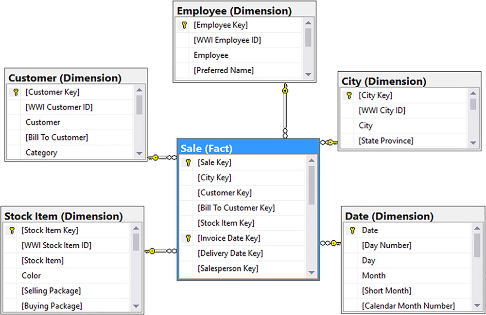
In an ideal data model for a multidimensional database, data is denormalized to minimize the number of joins across multiple tables by using a star schema, which consists of dimension tables and at least one fact table in which measures are stored. If you create a diagram by placing the fact table in the center and surround it by related dimensions, the diagram resembles a star shape, as shown in Figure 1-1. This example of a star schema is a selection of six tables from the WideWorldImportersDW sample database for SQL Server 2016 that answer some of the questions established as the requirements for the multidimensional database that you build throughout this chapter.
Note WideWorldImportersDW sample database
You can download the WideWorldImportersDW sample database from https://github.com/Microsoft/sql-server-samples/releases/tag/wide-world-importers-v1.0. Installation instructions are at https://msdn.microsoft.com/library/mt734217.aspx.
Although a star schema is not required as a source for SSAS, it is a preferred structure for enterprise-scale multidimensional models for several reasons. First, the impact of accessing the OLTP system from SSAS adds resource contention to your environment that you can avoid by creating a separate data source. (The degree of impact on the OLTP depends on the storage model you select as explained in the “Select a storage model” section in this chapter.) Second, the amount of time to move data from the OLTP system into the multidimensional database is sometimes less optimal than it can be if you restructure the data first. Third, sometimes analysis requires access to historical information that is no longer preserved in the source system. Having a separate data model in which you store data as it changes becomes a necessity in that case. Other reasons for creating a separate data model include, but are not limited to, cleansing data that cannot be corrected in the OLTP system, having the results available not only to the multidimensional database, but other downstream reporting systems (often with better performance than querying the OLTP directly), and integrating data from multiple OLTP systems.
Note Snowflake dimension design
Another type of design that you can implement for a dimension is a snowflake, in which you use multiple related tables for a single dimension. In traditional dimension modeling, the use of snowflake dimensions is not considered best practice because it adds joins back into the data model that a star schema design seeks to eliminate. For relational reporting scenarios, the additional joins can have an adverse impact on performance. However, when you use SSAS in its default storage mode, the snowflake structure has no impact on performance and can be a preferable design when you need to support analysis across fact tables having different levels of granularity, or to simplify the process that loads the dimension from the OLTP source. You can learn more about why you might use a snowflake dimension and how to design one properly in a series of blog posts by Jason Thomas that begins at http://sqljason.com/2011/05/when-and-how-to-snowflake-dimension.html.
To load the star schema with data on a periodic basis, you use an extract-transform-load (ETL) tool, such as SQL Server Integration Services (SSIS). The ETL tool is typically scheduled to run nightly to load new and changed rows into the star schema, although business requirements might dictate a different frequency, such as every five minutes when low latency is required, or once per week for source data that changes infrequently.
 Exam Tip
Because the focus of the 70-768 exam is on the implementation of Analysis Services models, this exam reference does not explain how to convert data from an OLTP structure such as Wide World Importers to a star schema structure suitable for OLAP. The assumption for the exam is that the design of the dimension and fact tables is complete and an ETL process has loaded the tables with data from the source OLTP system. Nonetheless, you should be familiar with star schema concepts and terminology and understand how to implement Analysis Services features based on specific data characteristics and analysis requirements.
A dimension table contains data about the entities that a business user wants to analyze—typically a person, place, thing, or point in time. One consideration when designing a dimension table is whether to track history. A slowly changing dimension (SCD) is a dimension for which you implement specific types of columns and ETL techniques specifically to address how to manage table updates when data changes. You make this design decision for each dimension separately based on business requirements. The two more common approaches to managing history include the following SCD types:
![]() Type 1 Only current data is tracked. The ETL process updates columns with changed values and loses the values previously stored in those columns. For example, you might not track history for employee name changes, as shown in Figure 1-2, because the effect on sales is not likely to be relevant.
Type 1 Only current data is tracked. The ETL process updates columns with changed values and loses the values previously stored in those columns. For example, you might not track history for employee name changes, as shown in Figure 1-2, because the effect on sales is not likely to be relevant.

![]() Type 2 Both current data and historical data is tracked. The ETL process expires the row containing the original data, thus identifying it as historical data, and creates a new active row containing the current data. When data in one of the columns changes in a row, the ETL process updates the Valid To date on the existing row to reflect the current date, and thus expires that record, and then adds a new record with the current values for each column and sets the Valid From date to the current date. Depending on the business rules, the Valid To date can be
Type 2 Both current data and historical data is tracked. The ETL process expires the row containing the original data, thus identifying it as historical data, and creates a new active row containing the current data. When data in one of the columns changes in a row, the ETL process updates the Valid To date on the existing row to reflect the current date, and thus expires that record, and then adds a new record with the current values for each column and sets the Valid From date to the current date. Depending on the business rules, the Valid To date can be NULL or a future date such as 12/31/9999.
As an example, you might track history for changes to a stock item’s data such as retail price, as show in Figure 1-3, because you might want to monitor whether sales change when the retail price changes.

Note Slowly changing dimension types
There are several different ways to model dimensions to accommodate changes besides Type 1 and Type 2, but these two are the most common. You can learn more about Type 1 from Ralph Kimball at http://www.kimballgroup.com/2008/08/slowly-changing-dimensions/ and about Type 2 at http://www.kimballgroup.com/2008/09/slowly-changing-dimensions-part-2/.
Let’s take a closer look at City, one of the dimension tables in the WideWorldImportersDW database, to understand the types of columns that it contains. Figure 1-2 shows the following types of columns commonly found in a dimension:
![]() Surrogate key A primary key for the dimension table to uniquely identify each row. It normally has no business meaning and is often defined as an identity column. In the City table, the [City Key] column is the surrogate key. The purpose of a surrogate key is to prevent duplicate rows when combining data from multiple sources or capturing historical data for slowly changing dimensions. In addition, the source data for a dimension table might not use an integer value for its primary key whereas enforcing an integer-based key in a dimension table ensures optimal performance when processing the dimension to load its data in a multidimensional database.
Surrogate key A primary key for the dimension table to uniquely identify each row. It normally has no business meaning and is often defined as an identity column. In the City table, the [City Key] column is the surrogate key. The purpose of a surrogate key is to prevent duplicate rows when combining data from multiple sources or capturing historical data for slowly changing dimensions. In addition, the source data for a dimension table might not use an integer value for its primary key whereas enforcing an integer-based key in a dimension table ensures optimal performance when processing the dimension to load its data in a multidimensional database.
Note Date dimension
It is not uncommon to see a date dimension without a surrogate key defined. Instead, an integer value for the date in YYYYMMDD format is used to uniquely identify each date. By using this approach, uniqueness is guaranteed. Furthermore, the issues with combining data sources or managing slowly changing dimensions do not occur in a date dimension.
![]() Natural or business key The primary key in the source table for the dimension, which is [WWI City ID] in the City table. This column is typically not displayed to business users for analytical purposes, but is used to match rows from the source system to existing rows in the dimension table as part of the ETL process.
Natural or business key The primary key in the source table for the dimension, which is [WWI City ID] in the City table. This column is typically not displayed to business users for analytical purposes, but is used to match rows from the source system to existing rows in the dimension table as part of the ETL process.
![]() Attributes Descriptive columns about a row in the dimension table. Attributes in the City table include City, State Province, Country, Continent, Sales Territory, Region, Subregion, Location, and Latest Recorded Population. Attributes can be used explicitly for analysis to aggregate numeric values from the fact table, much like you use a GROUP BY clause in a Transact-SQL (T-SQL) SELECT statement.
Attributes Descriptive columns about a row in the dimension table. Attributes in the City table include City, State Province, Country, Continent, Sales Territory, Region, Subregion, Location, and Latest Recorded Population. Attributes can be used explicitly for analysis to aggregate numeric values from the fact table, much like you use a GROUP BY clause in a Transact-SQL (T-SQL) SELECT statement.
![]() Slowly changing dimension history A pair of columns to show the date range for which a row is valid. Slowly changing dimension history columns specify the date range for which the set of attributes in the row is valid in a Type 2 SCD. In WideWorldImportersDW, Valid From and Valid To are the columns fulfilling this role. Another common naming convention is StartDate and EndDate.
Slowly changing dimension history A pair of columns to show the date range for which a row is valid. Slowly changing dimension history columns specify the date range for which the set of attributes in the row is valid in a Type 2 SCD. In WideWorldImportersDW, Valid From and Valid To are the columns fulfilling this role. Another common naming convention is StartDate and EndDate.
Note history tracking is optional
A Type 1 SCD dimension table for which only current data is tracked does not typically contain history columns.
Although the City table in WideWorldImportersDW is implemented as if it were a slowly changing dimension, because it includes history columns Valid From and Valid To, the data in the table does not reflect changed data across the historical records. Instead, you can observe an example of slowly changing dimension history in the Stock Item dimension table, which shows a change in Color that resulted in multiple rows for the WWI Stock Item ID 2, as shown in Figure 1-4.

Notice there are three surrogate keys, Stock Item Key, for the same natural key, and WWI Stock Item ID. Each surrogate key is associated with a separate range of Valid From and Valid To dates.
![]() Lineage or audit key An optional column in a dimension table that has a foreign key relationship to another table in which information about ETL processes is maintained. In WideWorldImportersDW, the City table, shown in Figure 1-5, has the Lineage Key column that relates to the Integration.Lineage table. This latter table includes the date and time when the ETL process started and ended, the table affected, and the success of the process.
Lineage or audit key An optional column in a dimension table that has a foreign key relationship to another table in which information about ETL processes is maintained. In WideWorldImportersDW, the City table, shown in Figure 1-5, has the Lineage Key column that relates to the Integration.Lineage table. This latter table includes the date and time when the ETL process started and ended, the table affected, and the success of the process.

A fact table contains many columns of numeric data. A business user analyzes the data in many of these columns in aggregate—typically by calculating sums, averages, or counts. Other numeric columns containing foreign keys are used to protect relational integrity with dimension tables through foreign key relationships. A fact table supports comparisons of these aggregate values over different time periods, such as this year’s total sales versus last year’s total sales, or across different groups, such as brands or colors of stock items. Figure 1-6 shows an example of Sale, a fact table in WideWorldImportersDW that contains the following types of columns:
![]() Surrogate key A primary key for the fact table to uniquely identify each row. Like a surrogate key for a dimension table, it normally has no business meaning and is often defined as an identity column. Often, a fact table has no surrogate key because the collection of foreign key columns represents a unique composite key. The inclusion of a surrogate key for a fact table is a matter of preference by the data modeler.
Surrogate key A primary key for the fact table to uniquely identify each row. Like a surrogate key for a dimension table, it normally has no business meaning and is often defined as an identity column. Often, a fact table has no surrogate key because the collection of foreign key columns represents a unique composite key. The inclusion of a surrogate key for a fact table is a matter of preference by the data modeler.
Note Benefits of a surrogate key in a fact table
Bob Becker, a member of the Kimball Group established by Ralph Kimball, recommends omitting a surrogate key in a fact table, but acknowledges it can be useful under special circumstances as he describes in his article on the topic at http://www.kimballgroup.com/2006/07/design-tip-81-fact-table-surrogate-key/.
![]() Foreign keys One foreign key column for each dimension table that relates to the fact table. In the Sale table, the following columns are foreign key columns for dimensions: City Key, Customer Key, Bill To Customer Key, Stock Item Key, Invoice Date Key, Delivery Date Key, and Salesperson Key. The combination of foreign keys represents the granularity, or level of detail, of the fact table.
Foreign keys One foreign key column for each dimension table that relates to the fact table. In the Sale table, the following columns are foreign key columns for dimensions: City Key, Customer Key, Bill To Customer Key, Stock Item Key, Invoice Date Key, Delivery Date Key, and Salesperson Key. The combination of foreign keys represents the granularity, or level of detail, of the fact table.
![]() Degenerate dimension One or more optional columns in a fact table that represents a dimension value that is not stored in a separate table. Technically speaking, the column can be stored in a separate table because it represents a “thing,” such as an invoice that could be the subject of analysis. Often the value in a degenerate dimension is unique in each row, such as an invoice identifier. However, due to the cardinality between the degenerate dimension and the fact table, the model is more efficient when the degenerate dimension is part of the fact table. In other words, no join is required to join two potentially large tables. An example of this type of degenerate dimension column in the Sale fact table is the WWI Invoice ID column.
Degenerate dimension One or more optional columns in a fact table that represents a dimension value that is not stored in a separate table. Technically speaking, the column can be stored in a separate table because it represents a “thing,” such as an invoice that could be the subject of analysis. Often the value in a degenerate dimension is unique in each row, such as an invoice identifier. However, due to the cardinality between the degenerate dimension and the fact table, the model is more efficient when the degenerate dimension is part of the fact table. In other words, no join is required to join two potentially large tables. An example of this type of degenerate dimension column in the Sale fact table is the WWI Invoice ID column.
Another reason to create a degenerate dimension in a fact table is to optimize reporting for frequently requested data by avoiding a join between tables. In the Sale fact table, the Description and Package columns are examples of this other type of degenerate dimension.
![]() Measure One or more columns that contain numeric data that describes an event or business process. The Sale fact table presents individual sales, so each row contains the following measure columns: Quantity, Unit Price, Tax Rate, Total Excluding Tax, Tax Amount, Profit, Total Including Tax, Total Dry Items, and Total Chiller Items.
Measure One or more columns that contain numeric data that describes an event or business process. The Sale fact table presents individual sales, so each row contains the following measure columns: Quantity, Unit Price, Tax Rate, Total Excluding Tax, Tax Amount, Profit, Total Including Tax, Total Dry Items, and Total Chiller Items.
Sometimes, a fact table contains no measure columns. In that case, it is known as a factless fact table. You might use a factless fact table when you need to count occurrences of an event and have no other measurements related to the event. Another type of factless fact table is a table that serves as a bridge table between a fact table and a dimension table, as described in the “Many-to-many dimension model” section in this chapter.
![]() Lineage or audit key An optional column in a fact table just like the same type of column in a dimension table. In the Sale table, Lineage Key is the lineage column.
Lineage or audit key An optional column in a fact table just like the same type of column in a dimension table. In the Sale table, Lineage Key is the lineage column.

Project creation
Once you have a star schema implemented and loaded with data, you are ready to create a project in which you perform the development of your multidimensional database. To do this, you use SSDT for which there is a link to the current version at https://msdn.microsoft.com/en-us/library/mt204009.aspx.
Note Location for SSDT download is subject to change
From time to time, Microsoft revises SSDT to update and fix features. If the referenced link is no longer valid, you can search for SQL Server Data Tools for Visual Studio at http://www.microsoft.com to locate and download it.
To create a new project, perform the following steps:
1. In the File menu, point to New, and then select Project.
2. In the New Project dialog box, select Analysis Services in the Business Intelligence group of templates, and then select Analysis Services Multidimensional and Data Mining Project.
3. At the bottom of the dialog box, type a name for the project, select a location, and optionally type a new name for the project’s solution. The project for the examples in this chapter is named 70-768-Ch1.
Note Solution structure in SSDT
A solution is a container for one or more projects. For example, you can have a data project to define your table structures, an SSIS project to perform the ETL steps, an Analysis Services project to create your multidimensional database, and a Microsoft SQL Server Reporting Services (SSRS) project to develop reports to display data from your multidimensional database.
Data source development
Your next step is to define a relational data source for your multidimensional database. SSAS supports the following data sources:
![]() Microsoft Access 2010 or higher
Microsoft Access 2010 or higher
![]() Microsoft SQL Server 2008 or higher
Microsoft SQL Server 2008 or higher
![]() Microsoft Azure SQL Database
Microsoft Azure SQL Database
![]() Microsoft Azure SQL Data Warehouse
Microsoft Azure SQL Data Warehouse
![]() Microsoft Analytics Platform System
Microsoft Analytics Platform System
![]() Oracle 9i or higher
Oracle 9i or higher
![]() Teradata V2R6 or V12
Teradata V2R6 or V12
![]() Informix V11.10
Informix V11.10
![]() IBM DB2 8.1
IBM DB2 8.1
![]() Sybase Adaptive Server Enterprise 15.0.2
Sybase Adaptive Server Enterprise 15.0.2
![]() A data source accessible by using an OLE DB provider
A data source accessible by using an OLE DB provider
Note Data provider installation
Depending on the data source that you are accessing, you might need to download and install the data source’s data provider on your computer. SSDT installation does not install data providers.
To add a data source, perform the following steps:
1. Right-click the Data Sources folder in the Solution Explorer window, and select New Data Source.
2. Click Next in the Data Source Wizard, and then click New on the Select How To Define The Connection page of the wizard.
3. In the Connection Manager dialog box, select a data provider and provide connection details for your data source. To follow the examples in this chapter, use the default provider, Native OLE DBSQL Server Native Client 11.0. Type your server name or type a period (.), (local), or localhost if you are running SSDT on the same computer as your SQL Server database engine. If you have your database set up for SQL Server authentication, select SQL Server Authentication in the Authentication drop-down list, and then provide a user name and password in the respective text boxes. Last, select WideWorldImportersDW in the Select Or Enter A Database Name drop-down list, as shown in Figure 1-7.

4. Click OK to close the Connection Manager dialog box, click Next in the Data Source Wizard, and then choose one of the following options for Impersonation Information, as shown in Figure 1-8, as authentication for the data source:
![]() Use Specific Windows User Name And Password Use this option when you need to connect to your data source with a specific login. A security best practice is to establish a Windows login with low privileges that has read permission to the data source. When you deploy the data source to the server, SSAS encrypts the password to protect it. If you later need to script out the database, such as you might when you want to move from a development server to a production server, you must provide the password again.
Use Specific Windows User Name And Password Use this option when you need to connect to your data source with a specific login. A security best practice is to establish a Windows login with low privileges that has read permission to the data source. When you deploy the data source to the server, SSAS encrypts the password to protect it. If you later need to script out the database, such as you might when you want to move from a development server to a production server, you must provide the password again.
![]() Use The Service Account To follow the examples in this chapter, the selection of this option is recommended. With this option selected, the account running the SSAS service, which by default is NT ServiceMSSQLServerOLAPService, is used to connect to the data source.
Use The Service Account To follow the examples in this chapter, the selection of this option is recommended. With this option selected, the account running the SSAS service, which by default is NT ServiceMSSQLServerOLAPService, is used to connect to the data source.
![]() Use The Credentials Of The Current User Do not select this option when you are developing a multidimensional database. It is included to support authentication for data mining queries.
Use The Credentials Of The Current User Do not select this option when you are developing a multidimensional database. It is included to support authentication for data mining queries.
![]() Inherit This option uses the impersonation information that is set for the DataSourceImpersonationInfo database property. Your options include Use A Specific Windows User Name And Password, Use The Service Account, Use The Credentials Of The Current User, or Default. If it is set to Default, the Inherit selection at the data source level uses the service account.
Inherit This option uses the impersonation information that is set for the DataSourceImpersonationInfo database property. Your options include Use A Specific Windows User Name And Password, Use The Service Account, Use The Credentials Of The Current User, or Default. If it is set to Default, the Inherit selection at the data source level uses the service account.

5. Click Next in the Data Source Wizard, change the value of the Data Source Name if you like, and then click Finish.
A new file is added to your project, Wide World Importers DW.ds. This file, like all the other files that you add to your project during the development process, is an Extensible Markup Language for Analysis (XMLA) file that defines the object to create in the multidimensional database. You can view the contents of any XMLA file by right-clicking it in the Solution Explorer window, and then selecting View Code.
Important Read permission for impersonation account
You should ensure that, whichever option you select for impersonation, the applicable login is granted the Read permission on the source database. Otherwise, when you later attempt to create the multidimensional database on the SSAS server, you receive an error message. If you configure writeback or ROLAP processing as described in Chapter 4, “Configure and maintain SQL Server Analysis Services (SSAS),” the account you use must also have write permission.
To set up read permission for the service account, open SQL Server Management Studio (SSMS), connect to the Database Engine, expand the Security node in Object Explorer, right-click the Logins node, and select New Login. In the Login dialog box, type NT SERVICEMSSQLServerOLAPService in the Login Name text box. Click the User Mapping page, select the WideWorldImportersDW check box in the Users Mapped To This Login section of the page, and then select the db_datareader check box in the Database Role Membership For: WideWorldImportersDW section of the page. Click OK to add the login.
Data source view design
The data source definition defines where the data is located and how to authenticate, but does not specify which data to use for loading into database objects, such as dimensions and cubes. A data source view (DSV) is the definition, which identifies the specific tables and columns within tables to use when populating the multidimensional database. It is also an abstraction layer that is useful when you have only read permission on the source database, or when you need a simplified view of its structures. You can make logical changes to the tables and views in the DSV to support specific requirements in SSAS without the need to change the physical data source. Generally speaking, you should attempt to change the physical data source as needed whenever possible because implementing logical changes in the DSV can introduce challenges into ongoing maintenance in addition to the troubleshooting process.
To create a DSV, perform the following steps:
1. Right-click the Data Source Views folder in Solution Explorer, and select New Data Source View.
2. In the Data Source View Wizard, click Next, select the data source that you created for the project in the previous section, and click Next.
3. Then, while pressing the CTRL key, select the following tables in the Available Objects list:
![]() City (Dimension)
City (Dimension)
![]() Customer (Dimension)
Customer (Dimension)
![]() Date (Dimension)
Date (Dimension)
![]() Employee (Dimension)
Employee (Dimension)
![]() Stock Item (Dimension)
Stock Item (Dimension)
![]() Sale (Fact)
Sale (Fact)
4. Then click the Right (>) arrow to add the selected tables to the Included Objects list.
5. Click Next, and then click Finish to complete the wizard. A new file, Wide World Importers DW.dsv, is added to the project, and Data Source View Designer is opened as a document window in SSDT, as shown in Figure 1-9.

When the source tables have primary keys and foreign key relationships defined, which is the ideal situation, the DSV includes them. If you are working with a well-defined star schema, the DSV probably does not require any modification.
If a primary key is not defined in a dimension table, either by design or because the source object is a view, you can add a logical key by right-clicking the column name in the table diagram or in the Tables pane, and then selecting Set Logical Primary Key. This command is not available when a key already exists for the table. If you press the CTRL key, and then select multiple columns, you can configure a composite key as the logical primary key.
To create a relationship between tables, such as between a fact table and a dimension table, click the foreign key column in the fact table and then drag it to the primary key column in the dimension table. The two columns must have the same data type before you can create the relationship. The definition of relationships is not required, but is useful because SSDT can make recommendations or automatically configure certain objects based on the DSV relationships that it detects.
The structure of the DSV is important for the development of dimension and cube objects as you continue building out your multidimensional database. To satisfy specific structural requirements for subsequent development steps, or to simplify a star schema, you can make any of the following changes to the DSV:
![]() Rename objects When you rename tables and columns in the DSV, the wizards that you use to create objects for the database reflect the new names, which should be a user-friendly name. Although you can later rename an object created by a wizard at any time, sometimes you might reference the same DSV object multiple times and can minimize the number of name changes required elsewhere in your project.
Rename objects When you rename tables and columns in the DSV, the wizards that you use to create objects for the database reflect the new names, which should be a user-friendly name. Although you can later rename an object created by a wizard at any time, sometimes you might reference the same DSV object multiple times and can minimize the number of name changes required elsewhere in your project.
![]() Create a named calculation The addition of a named calculation to a DSV is like adding an expression to a SELECT statement to add a derived column to a view. Ideally, when you need data structured in a particular way for SSAS, you design the source table to include that structure or create a view. A common reason to restructure data is to concatenate columns, such as you might need to do with First Name and Last Name columns to create one column for a person’s name.
Create a named calculation The addition of a named calculation to a DSV is like adding an expression to a SELECT statement to add a derived column to a view. Ideally, when you need data structured in a particular way for SSAS, you design the source table to include that structure or create a view. A common reason to restructure data is to concatenate columns, such as you might need to do with First Name and Last Name columns to create one column for a person’s name.
If you are unable to make the change in the source, create a named calculation in the DSV by right-clicking the header of the table to update, and selecting New Named Calculation. In the Create Named Calculation dialog box, type a name in the Column Name box, optionally type a description for the calculation in the Description box, and then type a platform-specific Structured Query Language (SQL) expression for the new column in the Expression box. There is no validation of the expression when you click OK to close the dialog box, so be sure to test your expression in a query tool first. You use the syntax applicable to the version of SQL applicable to your data source, such as Transact-SQL when your data source is SQL Server.
![]() Create a named query A named query in a DSV is the logical equivalent of a view in a relational database. Unlike a named calculation, which is limited to a SQL expression, a named query is a SELECT statement. You can use it to reduce the number of columns from a table to simplify the DSV, create new columns by using SQL expressions, or join tables together to simplify the data structures in the DSV and avoid a snowflake design. You can find examples of adding named queries to the DSV in Skill 1.2, “Design and implement dimensions in a cube,” and Skill 1.3, “Implement measures and measure groups in a cube.”
Create a named query A named query in a DSV is the logical equivalent of a view in a relational database. Unlike a named calculation, which is limited to a SQL expression, a named query is a SELECT statement. You can use it to reduce the number of columns from a table to simplify the DSV, create new columns by using SQL expressions, or join tables together to simplify the data structures in the DSV and avoid a snowflake design. You can find examples of adding named queries to the DSV in Skill 1.2, “Design and implement dimensions in a cube,” and Skill 1.3, “Implement measures and measure groups in a cube.”
Develop a dimension
A dimension in a cube is based on one or more dimension tables in a star schema. Skill 1.2 details the various options you must consider when developing different types of dimension models in SSAS. Regardless of model type, the development process for all dimensions begins by performing the same steps explained in this section.
Let’s review the basic dimension development process by adding the City dimension to the current database project. To this, perform the following steps:
1. Right-click the Dimensions folder in Solution Explorer, and click New Dimension.
2. In the Dimension Wizard, click Next on the first page, and then, on the Select Creation Method page, choose the Use An Existing Table option. Click Next.
Note Other dimension creation methods
The Select Creation Method page of the Dimension Wizard also allows you to choose one of the following alternatives to the default option: Generate A Time Table In The Data Source, Generate A Time Table On The Server, or Generate A Non-time Table In The Data Source. These options are used more often when you develop a prototype multidimensional database and have not built the star schema source tables. If you are interested in learning more about these options, see “Select Creation Method (Dimension Wizard)” at https://msdn.microsoft.com/en-us/library/ms178681.aspx.
3. On the Specify Source Information page of the wizard, select the name of the table containing the most granular level of detail for a dimension in the Main Table drop-down list. For the current example, select City. When the DSV is designed correctly, the key column in the source table displays automatically in the Key Columns list. The selection of a Name Column, such as City, as shown in Figure 1-10, is optional, but recommended when the key column is a surrogate key.

If you follow proper dimensional modeling design principles as described in the “Source table design” section earlier in this chapter, your key column is an integer value. If you do not specify a name column during dimension development, business users will see the dimension’s key column value when exploring a cube, which has no meaning to them. The Name Column should be set to a column in the dimension table that contains a meaningful value. Unlike the key column, which can be a composite key, the name column must reference a single column. If necessary, you can use a named calculation or named query to combine values from a multiple column into one column.
4. Click Next to continue. On the Select Dimension Attributes page of the Dimension Wizard, notice the existing selection of the City Key check box, and then select the check box for the following attribute columns, as shown in Figure 1-11:
![]() State Province
State Province
![]() Country
Country
![]() Continent
Continent
![]() Sales Territory
Sales Territory
![]() Region
Region
![]() Subregion
Subregion
![]() Latest Recorded Population
Latest Recorded Population

Note Additional options on the Select Dimension Attributes page of the Dimension Wizard
For each attribute on the Select Dimension Attributes page of the Dimension Wizard, you can select the Enable Browsing check box, or change the value in the Attribute Type drop-down list. For the current example, you can accept the default settings. When you develop your own multidimensional database, you can decide whether to change the defaults here, or to set the corresponding properties in the dimension definition as described in Skill 1.2. Selecting the Enable Browsing check box changes the dimension’s AttributeHierarchyEnabled property to False while changing the Attribute Type drop-down list selection updates the Type property for the attribute.
When business users analyze data by using a multidimensional model, they use attributes primarily for grouping aggregate values in a report, or to filter values, as shown in Figure 1-12. In this example, SSAS calculates the sum of the Sales Amount With Tax measure for each State Province attribute member appearing on rows. An attribute member is a distinct value from the source column that is bound to the attribute. Figure 1-12 shows attribute members for the State Province attribute such as Alaska, California, and so on. Above the set of State Province members, you can see a filter applied based on another attribute, Sales Territory. Specifically, the filter uses the Far West member of the Sales Territory attribute. SSAS ignores the values for any State Province attribute member that is not related to the Far West Sales Territory and eliminates those attribute members from the query results.

As explained earlier in the “Source table design” section, a dimension table can include columns that are never used for analysis, such as the Valid From and Valid To columns in the City dimension table. These columns are used for managing historical data in the ETL process, but are not useful for business analysis and are therefore normally excluded from the dimension in the SSAS project.
5. To complete the wizard, click Next, and then click Finish. The City.dim file is added to the project, and the dimension designer window is displayed in SSDT, as shown in Figure 1-13. The attributes that you selected in the wizard now appear in the Attributes pane of the Dimension Structure page of the dimension designer. In addition, a diagram of the source table displays in the Data Source View pane. After you develop a cube for the multidimensional database, you can add this newly created dimension to that cube. However, there might be additional steps to perform as part of the dimension development process to satisfy specific analysis requirements, as described next, and later in Skill 1.2.

When you create a dimension and then browse the members in the dimension, occasionally, a member named Unknown appears that does not exist in the source table. The addition of this member to a dimension is a feature in SSAS that gracefully accommodates data quality issues in a fact table. The Unknown member that SSAS creates does not correspond to a row in your dimension table, but serves as a bucket for values for which a key in the foreign key column in the fact table is missing or invalid. That way, when queries calculate totals for a measure, all rows in the fact table are included (after applying the applicable groupings and filters) even when they cannot be matched to existing dimension members.
The addition of the SSAS-generated member is determined by the value of the UnknownMember property for a dimension, which you can access in the Properties window from the Dimension Structure page of the dimension designer after selecting the dimension object in the Attributes pane. The member is added if the UnknownMember property value is Visible or Hidden. Either way, the grand total values for a dimension show the correct aggregated value for a fact table. When this property is set to Visible and your query includes the dimension’s members in the results, you can see the aggregated value for fact table rows with a missing or incorrect key for that dimension assigned to the Unknown member. When this property is set to Hidden, the Unknown member does not display in the query results, although the grand total correctly includes its values. However, hiding the Unknown member can be confusing to business users who might notice the aggregation of visible members does not equal the grand total. For this reason, it is not considered best practice to hide the Unknown member.
Important Working with the Unknown Member
In real-world practice, your ETL process should prevent the insertion of a row into a fact table if a dimension member does not already exist. If you review the dimension tables in the WideWorldImportersDW database, you can see an Unknown member with a surrogate key of 0 in each table. The addition of an Unknown member to a dimension is a common practice to handle data quality problems. When you manage missing dimension members for fact data in the ETL process, you should remove the Unknown member generated by SSAS. To do this, set the UnknownMember property value to None.
Exam Tip
Be prepared to answer questions about working with the Unknown Member on the exam. For more review on this topic, see “Defining the Unknown Member and Null Processing Properties” at https://msdn.microsoft.com/en-us/library/ms170707.aspx.
In Skill 1.2, we review specific usage scenarios that require additional development steps. Meanwhile, as a general practice for all dimensions that you develop, you should evaluate which, if any, of the following tasks are necessary:
![]() Rename objects For example, notice in the Attributes pane that there is a key icon next to City Key to designate it as the key attribute. In other words, this is the attribute that is referenced in the fact table. In the Dimension Wizard, you specified City Key as the key column and City as the name column. The attribute’s name is inherited from the key column name. In this case, the name City Key is not user-friendly because many business users might not understand what Key means. More generally, consider avoiding technical terms and naming objects by using embedded spaces, capitalization, and business terms to create user-friendly objects. To rename a dimension or an attribute, select it in the Attributes pane. You can either right-click the object, select Rename, and type the new name, or replace the Name property in the Attributes pane. In this case, rename the City Key attribute to City.
Rename objects For example, notice in the Attributes pane that there is a key icon next to City Key to designate it as the key attribute. In other words, this is the attribute that is referenced in the fact table. In the Dimension Wizard, you specified City Key as the key column and City as the name column. The attribute’s name is inherited from the key column name. In this case, the name City Key is not user-friendly because many business users might not understand what Key means. More generally, consider avoiding technical terms and naming objects by using embedded spaces, capitalization, and business terms to create user-friendly objects. To rename a dimension or an attribute, select it in the Attributes pane. You can either right-click the object, select Rename, and type the new name, or replace the Name property in the Attributes pane. In this case, rename the City Key attribute to City.
![]() Change the sort order Each attribute member has an OrderBy property that sets the default sort order that determines the arrangement of attribute members in a group, such as when you display many attribute members on rows in a pivot table. In most cases, the attribute members display in alphabetical order, but you can override this behavior if you have a column with values that define an alternate sort order. You can choose one of the following values for the OrderBy property.
Change the sort order Each attribute member has an OrderBy property that sets the default sort order that determines the arrangement of attribute members in a group, such as when you display many attribute members on rows in a pivot table. In most cases, the attribute members display in alphabetical order, but you can override this behavior if you have a column with values that define an alternate sort order. You can choose one of the following values for the OrderBy property.
![]() Key This value is the default for every attribute except the key attribute if you assigned it a name column in the Dimension Wizard because every attribute always has a key column, but optionally has a name column. The sort order is alphabetical if the key column is a string data type (Char or WChar), or numerical if the key column data type is not a string.
Key This value is the default for every attribute except the key attribute if you assigned it a name column in the Dimension Wizard because every attribute always has a key column, but optionally has a name column. The sort order is alphabetical if the key column is a string data type (Char or WChar), or numerical if the key column data type is not a string.
Note Sorting by Composite key
Remember that an attribute can have a composite key based on multiple columns. This capability can be used to advantage for sorting purposes. In Skill 1.2, you learn how to use composite keys to not only manage uniqueness for attribute members in the Date dimension, but also to control the sort order of those members.
![]() Name The sort order is set to Name for the key attribute by default when you specify a name column in the Dimension Wizard. Any attribute in a dimension can have separate columns assigned as the key column or name column, so you can define the sort order based on the name column if that is the case.
Name The sort order is set to Name for the key attribute by default when you specify a name column in the Dimension Wizard. Any attribute in a dimension can have separate columns assigned as the key column or name column, so you can define the sort order based on the name column if that is the case.
![]() AttributeKey You can also define the sort order for an attribute based on the key column value of another attribute, but only if an attribute relationship (described in Skill 1.2) exists between the two attributes. As an example, in an Account dimension, you can have an Account Name attribute that you want to sort by the related Account Number attribute rather than alphabetically by the account’s name.
AttributeKey You can also define the sort order for an attribute based on the key column value of another attribute, but only if an attribute relationship (described in Skill 1.2) exists between the two attributes. As an example, in an Account dimension, you can have an Account Name attribute that you want to sort by the related Account Number attribute rather than alphabetically by the account’s name.
![]() AttributeName This option is like the AttributeKey sort order, except that the ordering is based on the name column of the related attribute instead of the key column.
AttributeName This option is like the AttributeKey sort order, except that the ordering is based on the name column of the related attribute instead of the key column.
![]() Convert an attribute into a member property A member property is an attribute that is not used in a pivot table for placement on rows or columns, or as a pivot table filter, but is used instead for reporting purposes. For example, you can display sales by customer and include each customer’s telephone number in a report, but would not typically show sales by telephone number. You can also use a member property as a filter in an ad hoc MDX query.
Convert an attribute into a member property A member property is an attribute that is not used in a pivot table for placement on rows or columns, or as a pivot table filter, but is used instead for reporting purposes. For example, you can display sales by customer and include each customer’s telephone number in a report, but would not typically show sales by telephone number. You can also use a member property as a filter in an ad hoc MDX query.
In the City dimension, change the AttributeHierarchyEnabled property to False for the Latest Recorded Population attribute to convert it to a member property. When you do this, the attribute does not display with the other attributes in client applications, although you can still reference it in MDX queries. Its availability for use in reporting depends on the tool. As an example, you can display a member property as a tooltip when you hover your cursor over a related attribute in a Microsoft Excel pivot table.
![]() Group attribute members into ranges A less commonly used, but no less important, feature of SSAS is its ability to break down a large set of attribute members into discrete ranges. For example, if you have 100,000 customers, it is impractical for a user to add all customers at once to a pivot table. Instead, you can configure SSAS to create groups of customers by setting the DiscretizationBucketCount and DiscretizationMethod properties.
Group attribute members into ranges A less commonly used, but no less important, feature of SSAS is its ability to break down a large set of attribute members into discrete ranges. For example, if you have 100,000 customers, it is impractical for a user to add all customers at once to a pivot table. Instead, you can configure SSAS to create groups of customers by setting the DiscretizationBucketCount and DiscretizationMethod properties.
Note discretization configuration
You can find a thorough discussion about configuring the discretization properties by Scott Murray in “SQL Server Analysis Services Discretization” at https://www.mssqltips.com/sqlservertip/3155/sql-server-analysis-services-discretization/.
![]() Add translations Global organizations can build a single multidimensional database and then add translations to display captions for dimensions and attributes that are specific to a user’s locale. You can also optionally bind an attribute to columns containing translated attribute member names.
Add translations Global organizations can build a single multidimensional database and then add translations to display captions for dimensions and attributes that are specific to a user’s locale. You can also optionally bind an attribute to columns containing translated attribute member names.
Exam Tip
The WideWorldImportersDW database does not include translations, so you cannot explore this feature in the multidimensional database that you are building for this chapter. However, the exam is likely to test your knowledge on this topic. To learn more about adding translation definitions, see “Translations in Multidimensional Models (Analysis Services)” at https://msdn.microsoft.com/en-us/library/hh230908.aspx and “Defining and Browsing Translations” at https://msdn.microsoft.com/en-us/library/ms166708.aspx. Translations apply not only to dimensions, but also to cube captions as described in the Microsoft Developer Network (MSDN) article.
You can see examples of using translations if you explore the AdventureWorks Multidimensional Model for which you can find a download link and a ReadMe file that includes installation instructions at “Adventure Works 2014 Sample Databases” at http://msftdbprodsamples.codeplex.com/releases/view/125550.
A best practice in programming is to build code once, and then to reference that code many times. You might think that a similar best practice exists in SSAS. Let’s say that you have multiple SSAS servers set up in your company to support different departments, and host different multidimensional databases on each server. If you follow dimensional modeling best practices, you have conformed dimensions in your data mart. That is, you have dimension tables that you relate to different fact tables, such as a Date dimension that is common to all analysis. If you build a date dimension for use in one multidimensional database, why not use the same dimension object in the other multidimensional database? SSAS allows you to add a linked dimension to that other multidimensional database so that you only have one dimension to build and maintain. However, the use of linked dimensions is not considered to be best practice in SSAS development because it can introduce performance problems in large cubes.
Note Linked dimensions and alternative development practices
Another way to think about building once and reusing your development work is to save the .dim files in source control. You can then require new multidimensional database projects to add .dim files from source control rather than build a new dimension directly. That way, you can maintain the design in a central location and benefit from reusability without introducing potential performance issues.
If you still want to learn more about working with linked dimensions, see “Define Linked Dimensions” at https://msdn.microsoft.com/en-us/library/ms175648.aspx.
Develop a cube
A cube is the object that business users explore when interacting with a multidimensional database. It combines measure data from fact tables with dimension data. At minimum, you associate a single fact table with a cube, although it is common to associate multiple fact tables with one cube.
Like dimension development, cube development begins by using a wizard. To add a cube to your project, perform the following steps:
1. Launch the Cube Wizard by right-clicking the Cubes folder in Solution Explorer, and selecting New Cube.
2. Click Next on the first page of the wizard, keep the default option, Use Existing Tables, and then click Next.
Note Other cube creation methods
The Select Creation Method page of the Cube Wizard also allows you to choose one of the following alternatives to the default option: Create An Empty Cube or Generate Tables In The Data Source. Just like dimension creation methods, these additional options are typically used when you develop a prototype multidimensional database and do not yet have the star schema source tables available. To learn more about these options, see “Select Creation Method (Cube Wizard)” at https://msdn.microsoft.com/en-us/library/ms187975.aspx.
3. On the Select Measure Group Tables page of the wizard, select a fact table, such as Sale, and then click Next. In SSAS, a measure group table is synonymous with a fact table. The reason for a more generic term is due to the ability to create a measure group from any type of table as long as it contains rows that can be counted. Therefore, think about a measure group as a container of measures.
4. On the Select Measures page of the Cube Wizard, only columns with a numeric data type in the fact table are displayed. Clear each check box that you do not want to use for analysis, such as WWI Invoice ID and Lineage Key in this example, as shown in Figure 1-14. Notice the inclusion of Sale Count, which is not a column in the fact table. SSAS suggests this column because counting the number of rows in a fact table and grouping the result by dimension attributes is a common business requirement. You can clear the check box for this derived measure if it is not necessary in your own project.

5. Click Next to continue to the Select Existing Dimensions page of the wizard. As shown in Figure 1-15, this page displays dimensions that currently exist in the project.

A common development approach is to build one dimension, build a cube, deploy the project, and then review the results. (Troubleshooting any problems that arise is easier when you deploy one object at a time.) You then continue iteratively by defining another dimension, adding it to the cube, deploying the project, and then reviewing the changes.
However, you can decide to define multiple dimensions first. If you do, you see the available dimensions listed here and can include or exclude them as needed when using the Cube Wizard. On the other hand, when you create dimensions after you complete the Cube Wizard, you follow different steps to add them to the cube as explained in Skill 1.2.
6. Click Next, and then, on the Select New Dimensions page of the wizard, clear all of the check boxes, as shown in Figure 1-16, to continue the current example in which you are developing a simple cube with one dimension. You can do this in one step by clearing the Dimension check box at the top of the page.

The purpose of this page in the wizard is to identify dimension tables for which a relationship exists with the fact table or tables selected for the cube. If you keep a table selected on this page, the Cube Wizard creates a basic dimension for that table and adds it to the project as a new .dim file. You can then configure the dimension’s properties as needed to meet your analysis requirements.
7. To finish the wizard, click Next, and then click Finish to add the Wide World Importers DW.cube file to the project and display the cube designer as an SSDT window.
8. Expand Sale in the Measures pane of the Cube Structure page of the cube designer to see all of the measures added to the cube, as shown in Figure 1-17.

The cube designer also includes a Dimensions pane that displays the one dimension that is included in the cube, City. In addition, the Data Source View pane displays a diagram of the fact table, displayed with a yellow header, and the related dimension table, displayed with a blue header.
Important Design warnings
Whenever you see a blue wavy underscore in a designer, you can hover your cursor over it to view the text of a design warning. In this case, the cube in both the Measures and Dimensions pane is associated with the same warning: Avoid cubes with a single dimension. Design warnings exist to alert you to potential problems that can affect performance or usability. Because it is a warning only, you can create your multidimensional database successfully if you ignore the warning. As you gain experience in developing multidimensional models, you can determine which warnings you should address, and which to ignore on a case-by-case basis. For more information about working with design warnings, see “Warnings (Database Designer) (Analysis Services-Multidimensional Data)” at https://msdn.microsoft.com/en-us/library/bb677343.aspx.
Create a multidimensional database
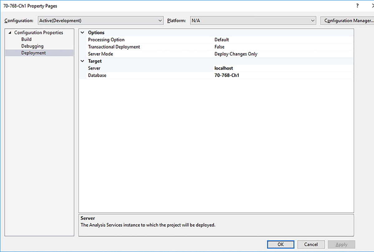
At this point, you have created the definitions of a data source, a data source view, a dimension, and a cube, which exist only in the context of a project, but the database does not yet exist on the server and no one can explore the cube until it does. To create the database on the server, you must deploy the project from SSDT. To ensure you deploy the project to the correct server, review, and if necessary, update the project’s properties. To do this, right-click the project name in Solution Explorer and select Properties. In the 70-768-Ch1 Property Pages dialog box, select the Deployment page, as shown in Figure 1-18, and then update the Server text box with the name of your SSAS server if you need to deploy to a remote server rather than locally.
The following additional deployment options are also available on this page:
![]() Processing Option The default value is Default, which evaluates the processed state of each object in the solution and takes the necessary steps to put the object into a processed state when you deploy the project. You can change this value to Do Not Process if you want to manually instruct the server to process objects as a separate step, or Full if you want the database to process completely each time you deploy your project from SSDT. For now, the default value is sufficient for working through the examples in this chapter. In Chapter 4, these processing options are described in greater detail.
Processing Option The default value is Default, which evaluates the processed state of each object in the solution and takes the necessary steps to put the object into a processed state when you deploy the project. You can change this value to Do Not Process if you want to manually instruct the server to process objects as a separate step, or Full if you want the database to process completely each time you deploy your project from SSDT. For now, the default value is sufficient for working through the examples in this chapter. In Chapter 4, these processing options are described in greater detail.
![]() Transactional Deployment The default value is False, which means that deployment is not transactional. In that case, deployment can succeed, but processing can fail. Choose True if you want to roll back deployment if processing fails.
Transactional Deployment The default value is False, which means that deployment is not transactional. In that case, deployment can succeed, but processing can fail. Choose True if you want to roll back deployment if processing fails.
![]() Server Mode The default value is Deploy Changes Only, which deploys only objects from your project that do not yet exist on the server, or are different from those on the server. This option is faster than the Deploy All option, which deploys all objects in your project to the server.
Server Mode The default value is Deploy Changes Only, which deploys only objects from your project that do not yet exist on the server, or are different from those on the server. This option is faster than the Deploy All option, which deploys all objects in your project to the server.
When you are ready to create the database on the server, right-click the project in Solution Explorer, and select Deploy. The first time you perform this step, the deployment process creates the database on the server and adds any objects that you have defined in the project. Each subsequent time that you deploy the project, as long as you have kept the default deployment options in the project properties, the deployment process preserves the existing database and adds any new database objects, and updates any database objects that you have modified in the project.
You can confirm the creation of the multidimensional database by opening SSMS and connecting to Analysis Services. In Object Explorer, expand the Databases folder to view the existing databases, and then expand the subfolders to see the objects currently in the database, as shown in Figure 1-19.

FIGURE 1-19 Multidimensional database objects visible in the SQL Server Management Studio Object Explorer
Now the cube is ready to explore using any tool that is compatible with SSAS, such as Excel, Microsoft Power BI Desktop, or SSRS, but it is not yet set up as well as it can be. There are more dimensions and fact tables to add, as well as many configuration changes to the dimension and cube to consider and implement that you learn about in Skills 1.2 and 1.3.
Important Example database focuses on exam topics
The remainder of this chapter describes many more tasks that you perform during the development of a multidimensional database. Some of these tasks are always necessary, while others depend on business requirements. If you follow all the steps described in this chapter to produce the 70-768-Ch1 multidimensional database, the resulting database is not as complete as it could be, and in some cases, it is contrived to demonstrate a technique because its purpose is to illustrate the topics that you must understand for the exam. Bringing the example multidimensional database to its best state is out of scope for this book.
For your own projects, be sure to explore the cube thoroughly and encourage business users to help you test the results. Start by reviewing the naming conventions of dimensions, attributes, hierarchies, measure groups, and measures. Make sure attribute members sort in a sequence that makes sense to your users. Check the aggregate values as you slice and dice the data by using various combinations of dimensions and attributes and compare these values to comparable SQL queries in the data source.
Select a storage model
The storage model you select for your multidimensional model determines the type of data that SSAS stores and how it physically stores that data on disk. SSAS supports the following storage models:
![]() Multidimensional OLAP (MOLAP)
Multidimensional OLAP (MOLAP)
![]() Relational OLAP (ROLAP)
Relational OLAP (ROLAP)
![]() Hybrid OLAP (HOLAP)
Hybrid OLAP (HOLAP)
Regardless of which storage model you select, cube data is always stored separately from dimension data. Furthermore, you can specify a different storage model for cube data than you do for dimension data. You can even separate cube data into multiple partitions, each using a different storage model. For now, consider which storage mode is most appropriate for your requirements in general. In Chapter 4, you learn the reasons why you might configure different storage models for partitions and how to implement storage models by partition.
Exam Tip
Be prepared to answer questions on the exam related to the selection of an appropriate storage model for a specific scenario. In addition, review the information in Chapter 4 to understand how proactive caching affects data latency.
MOLAP
MOLAP is the default storage mode. Generally speaking, it is also the preferred storage mode unless you have specific requirements that only one of the other two storage modes can meet because it performs fastest. On the other hand, it requires the most storage space.
MOLAP storage compresses data and distributes it more efficiently on disk than the other storage models, but it also requires the most time to process data. When SSAS processes data for MOLAP storage, it uses the DSV to generate the necessary SQL statements that retrieve data from the relational source, restructures the results for storage on disk in a proprietary format, and then calculates and stores aggregations for measures, as shown in Figure 1-20. Aggregations are calculated only if you have defined aggregation rules as described in Chapter 4. When SSAS receives a request for data from a Multidimensional Expression (MDX) query, it gets the aggregated data or detail data in MOLAP storage to prepare the results.

Note Data retrieval for MDX queries
More precisely, SSAS retrieves data from MOLAP storage if the data is not currently in memory. SSAS uses both disk and cache storage for managing multidimensional data. For the purposes of contrasting storage models, assume that the data for a query is not available in memory and must be retrieved from the applicable storage model. Chapter 4, delves deeper into the mechanics of query processing by explaining the relationship between disk and cache storage.
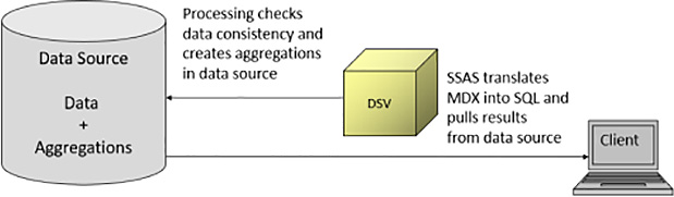
ROLAP
With ROLAP storage, SSAS does not retrieve data from the relational source during processing. Instead, processing involves only checking the consistency of the data and therefore runs much faster than MOLAP processing. If you configure aggregations in addition to ROLAP storage, the aggregated values are stored in the data source, as shown in Figure 1-21. When SSAS receives an MDX request for data, it uses the DSV to translate the request into an SQL statement and sends that statement to the data source. For example, if the data source is SQL Server, the MDX is translated into T-SQL.
ROLAP storage is the best choice when your business users require near real-time access to data or when a dimension table has hundreds of millions of rows. A potential trade-off is slower query performance due to the translation of the query from MDX to SQL. However, there are techniques you can apply to mitigate the performance degradation as explained in Chapter 4.
Note ROLAP dimension configuration
To configure a dimension to use ROLAP storage, open the dimension designer and select the dimension object in the Attributes pane. In the Properties windows, select ROLAP in the StorageMode property’s drop-down list. You learn how to configure ROLAP for measure group partitions in Chapter 4.
HOLAP
HOLAP storage is a combination of MOLAP and ROLAP. Detail data is kept in the relational data source, but aggregate data and indexes are loaded into MOLAP storage during processing, as shown in Figure 1-22. When SSAS processes an MDX query, it determines where the data necessary to resolve the query resides. If it needs detail data, it translates the query to SQL and sends the translated statement to the data source. Otherwise, it retrieves aggregated data from MOLAP storage.
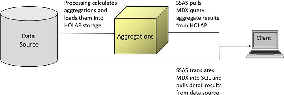
HOLAP queries are potentially slower to resolve. Furthermore, storage requirements on the SSAS server are not truly lower because SSAS must read all the data from the data source to build the aggregations and indexes and requires enough space to do this. SSAS disposes of the data afterwards, thus reducing storage requirements. Because you must factor in enough storage overhead for processing, HOLAP is not a good choice if your goal is to minimize storage.
Note HOLAP storage does not apply to dimensions
You can configure a dimension to use MOLAP or ROLAP storage only. HOLAP storage applies only to cube partitions.
Skill 1.2: Design and implement dimensions in a cube
After using the Dimension Wizard to add a dimension object to your multidimensional database, you must then add it to one or more cubes to make it available to client applications. Additionally, there are some configuration steps to perform when you need to improve the user experience for browsing the cube, enable specific SSAS features, or optimize performance.
Select an appropriate dimension model, such as fact, parent-child, roleplaying, reference, data mining, many-to-many, and slowly changing dimension
There are several different types of dimension models that you can define for your multidimensional database. For some of the dimensional models, you define the type by configuring its dimension usage relationship type on the Dimension Usage page of the cube designer. For the other dimensional models, you configure dimension or cube properties. In this section, we review each type of dimension model and the steps required to configure it.
Regular dimension model
When a dimension does not meet the criteria for any of the other dimensional models described in this section, it is considered to be a regular dimension. When you add it to a cube, the existence of a foreign key relationship between its corresponding dimension table and a measure group’s fact table usually results in the addition of a regular relationship type. Sometimes, for various reasons, you might need to add this relationship type manually.
You can confirm the existence of a regular relationship by reviewing dimension usage. To do this, perform the following steps:
1. In Solution Explorer, double-click Wide World Importers DW.cube to open the cube designer, and then click the Dimension Usage tab. When you see text displayed without an icon in the cell intersection between a dimension and a measure group, as shown in Figure 1-23, the relationship type is Regular.
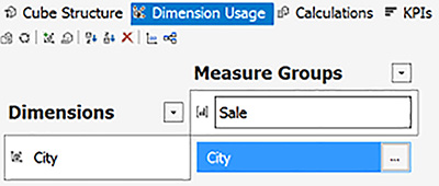
2. Click the ellipsis button in the cell intersection to open the Define Relationship dialog box, shown in Figure 1-24.

When Regular is selected in the Select Relationship Type drop-down list, you must identify the granularity attribute in the dimension, and the corresponding column in the measure group table.
In the Granularity Attribute drop-down list, you can select any attribute that exists in the dimension object in your project. This list does not include attributes from the dimension table appearing in the DSV if those attributes are not added to the dimension object.
When you select a granularity attribute, the attribute’s corresponding key columns in the dimension table, as defined in the dimension object, display in the Dimension Columns list at the bottom of the dialog box. You then match each key column to a foreign key column in the fact table associated with the measure group.
Think of dimension usage for a regular relationship as the SSAS definition of a foreign key relationship. The existence of that relationship in the DSV is not sufficient because that is used whenever SSAS needs to generate SQL statements during processing, or when translating MDX to SQL. The DSV represents the physical modeling of the data source, even if it includes derived elements. The purpose of dimension usage is to define the logical relationships between dimension and measure groups objects. It represents the logical modeling of your multidimensional database.
Fact dimension model
A fact dimension model allows you to define a relationship between a measure group and dimension object that you create from a degenerate dimension. Remember from Skill 1.1 that a degenerate dimension is a type of column found in a fact table. Because both the measure group and the dimension come from the same table, there is no additional configuration required after you specify the Fact relationship type.
Let’s set up a new dimension, configure a fact dimension model, and check the results by following these steps:
1. In Solution Explorer, right-click the Dimensions folder, select New Dimension, and click Next twice to proceed to the Specify Source Information page of the wizard.
2. In the Main Table drop-down list, select Sale.
The two primary keys in the Sale table display in the Key Columns list, which requires you to select an item in the Name Column list. However, there is no column that adequately represents a value for each row in this table and the invoice date is not required to uniquely identify each row in the table. Therefore, you can clear this value.
3. Open the drop-down list containing Invoice Date Key, scroll to the top of the list, and then select the blank row at the top of the list to remove Invoice Date Key. Now you no longer need to provide a Name Column value, so click Next to continue.
4. On the Select Related Tables page, clear each check box, and click Next.
5. On the Select Dimension Attributes page, select the check box to the left of WWI Invoice ID, scroll down, and clear the check boxes for Delivery Date Key, Stock Item Key, Invoice Date Key, Salesperson Key, Customer Key, City Key, and Bill To Customer Key, and then click Next.
6. Type Invoice in the Name box, and click Finish to complete the wizard.
7. In the Attributes pane, click Sale Key to highlight it. Then, in the Properties window, select False in the AttributeHierarchyVisible drop-down list.
By setting this property to False, you render the Sale Key attribute inaccessible to business users when they browse the cube. As a surrogate key, it has no meaning for business analysis, but is required in the dimension to uniquely identify each row and to establish the fact relationship in dimension usage.
8. Rename the WWI Invoice ID attribute by right-clicking it in the Attributes pane, selecting Rename, and then typing Invoice.
9. Double-click the Wide World Importers DW.cube file in Solution Explorer, go to the Cube Structure page, right-click the white space in the Dimensions pane, select Add Cube Dimension, select Invoice, and click OK. Now the dimension in the project is included in the cube.
10. Click the Dimension Usage tab of the cube designer, click the cell labeled Sale Key, and click the ellipsis button in the cell.
11. In the Define Relationship dialog box, select Fact in the Select Relationship Type drop-down list, as shown in Figure 1-25. There is nothing else to configure because the column for the granularity attribute for the dimension is also a column in the fact table for the measure group.
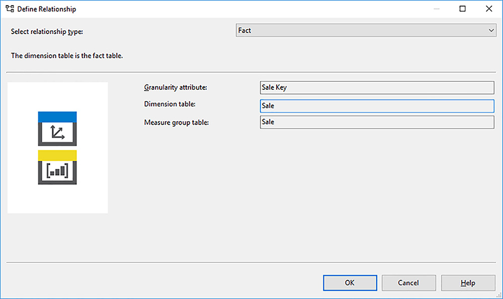
12. Click OK to close the dialog box. An icon displays in the Sale Key cell to indicate the fact relationship between the Invoice dimension and the Sale measure group.
13. Right-click the project in Solution Explorer, and select Deploy.
14. After the Deployment Completed Successfully message displays, click the Browser tab in the cube designer, expand the Measures node in the cube metadata tree, expand the Sale folder, and drag Sale Count to the query window labeled Drag Levels Or Measures Here To Add To The Query.
15. Expand the Invoice node, and drag Invoice (next to the rectangular collection of blue squares) to the area next to Sale Count. The browser generates an MDX query behind the scenes and displays the results, as shown in Figure 1-26. Here you can see some invoices have only one item sold, while others have multiple items sold. As you add dimensions to the cube, you can create a query to see the specific stock items sold, the salesperson selling the item, and more.

Parent-child dimension model
You use a parent-child dimension model when you have a dimension table that includes a foreign-key relationship to itself. It is also referred to as a ragged hierarchy or self-referencing relationship. Unlike a standard hierarchical structure in which there are a fixed number of levels, such as Month, Quarter, and Year in a Date dimension, a ragged hierarchy can have varying numbers of levels for each node. Common examples of ragged hierarchies are organizational charts, financial charts of accounts, or bills of materials.
Exam Tip
A ragged hierarchy can be a standard or a parent-child dimension structure. For the exam, you should know how to use the HideMemberIf property to manage navigation across levels of a ragged hierarchy as described in “Ragged Hierarchies” at https://msdn.microsoft.com/en-us/library/ms365406.aspx. Xian Wang has a blog post entitled “Ragged Hierarchies and HideMemberIf: an in-depth look” that illustrates your options for modeling ragged hierarchies at https://xzwang.wordpress.com/2013/07/10/ragged-hierarchy-and-hidememberif/. You should also review Chris Webb’s commentary on ragged hierarchy behavior in his blog post “Ragged Hierarchies, HideMemberIf and MDX Compatibility” at https://blog.crossjoin.co.uk/2009/11/11/ragged-hierarchies-hidememberif-and-mdx-compatibility/.
The WideWorldImportersDW database does not include a parent-child dimension, but you can artificially create one by converting the Employee table in the DSV to a named query in which you arbitrarily assign employees to managers. To do this, double-click Wide World Importers DW.dsv in Solution Explorer to open the DSV designer. In the Tables pane, right-click the Employee table, point to Replace Table, and select With New Named Query. In the Create Named Query dialog box, replace the SELECT statement with the statement shown in Listing 1-1, as shown in Figure 1-27, and then click OK.
LISTING 1-1 Named query statement to arbitrarily assign managers to employees
SELECT
[Employee Key],
CASE
WHEN [WWI Employee ID] >= 3 AND [WWI Employee ID] <= 11 THEN 194
WHEN [WWI Employee ID] >= 12 AND [WWI Employee ID] <= 15 THEN 203
WHEN [WWI Employee ID] >= 16 AND [WWI Employee ID] <= 19 THEN 208
WHEN [WWI Employee ID] = 20 THEN 210
ELSE NULL
END AS [Manager Key],
[WWI Employee ID],
[Employee],
[Preferred Name],
[Is Salesperson]
FROM [Dimension].[Employee];

Next, create the Employee dimension in the project by first following the steps described in the “Develop dimension” section earlier in this chapter and then performing these steps:
1. In the Specify Source Information page of the Dimension Wizard, use Employee as the Main Table and set Employee Key as the Key Column, and Employee as the Name Column. Click Next.
2. In the Select Dimension Attributes page of the wizard, select the Manager Key check box. Then click Next, and click Finish.
3. In the Attributes pane of the dimension designer, rename Employee Key as Employee, and Manager Key as Employees.
4. With Employees selected, locate the Usage property in the Properties window, and then select Parent in the Usage drop-down list. After you set this property, an icon displays next to the Employees attribute to designate its status as a parent-child hierarchy.
5. To observe the effect of this change, right-click the project in Solution Explorer, and select Deploy to update the multidimensional database on the server with the new dimension.
6. When you see the message the deployment is complete, click the Browser page of the dimension designer, and select Employees in the Hierarchy drop-down list.
7. Expand the All member in the browser, and then expand each member with a plus symbol next to it to view the parent-child hierarchical structure, as shown in Figure 1-28. In the Employees table in the WideWorldImportersDW table, there are multiple rows for many employees due to its slowly changing dimension design, which results in the appearance of duplicates in the dimension browser. You can safely ignore these duplicates for the purposes of this example.

When you create a parent-child dimensional model and set an attribute’s Usage property to Parent, you can also optionally configure the following additional properties for that attribute:
![]() MembersWithData The default setting for this property is NonLeafDataVisible. The assumption with this setting is that the fact table’s key column associated with this dimension contains values for both parent and child members. In the case of the WideWorldImportersDW data (after creating a contrived relationship for managers and employees in the named query), that means managers and employees are associated with rows in the fact table, such as Archer Lamble and Jack Potter. When you browse the cube, when you drill down to break out the total sales for Archer Lamble, you see it includes Archer’s sales reported as a separate value from Jack’s sales (which you can see if you drill down from Jack’s manager Katie Darwin).
MembersWithData The default setting for this property is NonLeafDataVisible. The assumption with this setting is that the fact table’s key column associated with this dimension contains values for both parent and child members. In the case of the WideWorldImportersDW data (after creating a contrived relationship for managers and employees in the named query), that means managers and employees are associated with rows in the fact table, such as Archer Lamble and Jack Potter. When you browse the cube, when you drill down to break out the total sales for Archer Lamble, you see it includes Archer’s sales reported as a separate value from Jack’s sales (which you can see if you drill down from Jack’s manager Katie Darwin).
If you change this property to NonLeafDataHidden, the totals for each manager are calculated correctly. However, you do not see the manager’s data in the query results when you drill down to view the employees’ sales for that manager. This behavior can be confusing to business users and is not recommended as a best practice.
Important Testing the effect of the MembersWithData attribute property
Although you can view the relationship between parent and child attribute members by using the Browse page of the dimension designer, you cannot view the effect of modifying the MembersWithData attribute property until you add the dimension to the cube, ensure the relationships on the Dimension Usage page of the cube designer is correct, and process the cube. Then you can browse the cube and use the parent attribute of the dimension in your query to see its behavior.
![]() MembersWithDataCaption If you use the NonLeafDataVisible setting for the MembersWithData property, you can set the caption for the attribute member that displays when you drill from the parent to the child attribute members. If you leave this property blank, the caption for both parent and child is identical. To more clearly differentiate the parent member as an aggregate value and its corresponding child member, you can use an asterisk as a wildcard and a string value to combine the actual member name with a static string.
MembersWithDataCaption If you use the NonLeafDataVisible setting for the MembersWithData property, you can set the caption for the attribute member that displays when you drill from the parent to the child attribute members. If you leave this property blank, the caption for both parent and child is identical. To more clearly differentiate the parent member as an aggregate value and its corresponding child member, you can use an asterisk as a wildcard and a string value to combine the actual member name with a static string.
As an example, you can type * (Manager) in the MembersWithData Caption. For the WideWorldmportersDW named query in this chapter’s sample project, Archer’s sales as a parent member is the aggregate value of sales made by Archer and Jack and displays as Archer Lamble. If you drill down, you see Archer’s sales as a child member displayed as Archer Lamble (Manager).
![]() NamingTemplate You use this property when you want to assign level names to each level in a parent-child hierarchy, which is important when your users browse the cube by using Excel or Power BI. If you leave this property blank, SSAS assigns a level names like Level 01, Level 02, and so on.
NamingTemplate You use this property when you want to assign level names to each level in a parent-child hierarchy, which is important when your users browse the cube by using Excel or Power BI. If you leave this property blank, SSAS assigns a level names like Level 01, Level 02, and so on.
In a standard hierarchy, you define the level names when you create the hierarchy, as explained later in this chapter in the “Define attribute relationships” section. If you want to provide a name for levels in a parent-child hierarchy, your only option is to use the naming template.
A parent-child hierarchy does not have a fixed number of levels, and each branch of the hierarchy tree can have zero to many different levels. The second level down one branch does not necessarily have the same context as the second level down another branch. For example, in the Employee dimension, Archer Lamble is a manager on the first level below the All member, and the second level below Archer includes Jai Shand, Katie Darwin, and Piper Koch. Let’s say hypothetically that each of these employees is a customer service representative. However, another member on the first level is Kayla Woodcock and the child members on the second level of this branch of the hierarchy are all sales staff. Therefore, it does not make sense to use a naming template in this scenario where the second level varies by branch.
When you have a parent-child hierarchy with a more consistent structure, you can use the NamingTemplate property to define a unique string for each level of the hierarchy. On the bottom level in the template, append an asterisk to the name to instruct SSAS to add a number that increments by 1 for each subsequent level when there are more levels in the hierarchy than named levels in the template.
![]() RootMemberIf You use this property to help SSAS distinguish parent members from child members. You can choose from one of the following values in the property’s drop-down list.
RootMemberIf You use this property to help SSAS distinguish parent members from child members. You can choose from one of the following values in the property’s drop-down list.
![]() ParentIsBlankSelfOrMissing This is the default setting, which covers any possible scenario to define a parent member. SSAS looks in the column defined as the parent key column, which is the attribute with the Usage property set to Parent, and if that column is blank, contains the same value as the dimension’s key attribute column, or is not also found in the dimension’s key attribute column on another row, the member is flagged as a parent member at the top level of the hierarchy. In other words, the member displays as the first level of members below the All member.
ParentIsBlankSelfOrMissing This is the default setting, which covers any possible scenario to define a parent member. SSAS looks in the column defined as the parent key column, which is the attribute with the Usage property set to Parent, and if that column is blank, contains the same value as the dimension’s key attribute column, or is not also found in the dimension’s key attribute column on another row, the member is flagged as a parent member at the top level of the hierarchy. In other words, the member displays as the first level of members below the All member.
![]() ParentIsBlank You use this setting when you want SSAS to consider a member as a parent only when the parent attribute column is blank.
ParentIsBlank You use this setting when you want SSAS to consider a member as a parent only when the parent attribute column is blank.
![]() ParentIsSelf You use this setting when you want SSAS to define a parent only when the parent attribute column matches the value in the key attribute column.
ParentIsSelf You use this setting when you want SSAS to define a parent only when the parent attribute column matches the value in the key attribute column.
![]() ParentIsMissing You use this setting when SSAS should identify a parent based on a parent attribute column value is not found anywhere in the table in the key attribute column.
ParentIsMissing You use this setting when SSAS should identify a parent based on a parent attribute column value is not found anywhere in the table in the key attribute column.
![]() UnaryOperatorColumn This property is used only for special design scenarios, such as a financial account dimension in which you need to change the default rollup behavior. Although many data warehouse developers opt to use positive and negative values in a financial fact table to manage rollup behavior for account balances, another less commonly used option is to include a column in the financial account dimension to contain operators that define this behavior. For example, when you want to compute a parent account member’s aggregate value, such as Income (Loss), you typically want to subtract one of its children, Expenses, from another of its children, Revenue. That is, Income (Loss) equals Revenue minus Expenses. You must include a value, such as a plus or minus symbol, in a column in your dimension table, and then map that column to the UnaryOperatorColumn property to define the rollup behavior.
UnaryOperatorColumn This property is used only for special design scenarios, such as a financial account dimension in which you need to change the default rollup behavior. Although many data warehouse developers opt to use positive and negative values in a financial fact table to manage rollup behavior for account balances, another less commonly used option is to include a column in the financial account dimension to contain operators that define this behavior. For example, when you want to compute a parent account member’s aggregate value, such as Income (Loss), you typically want to subtract one of its children, Expenses, from another of its children, Revenue. That is, Income (Loss) equals Revenue minus Expenses. You must include a value, such as a plus or minus symbol, in a column in your dimension table, and then map that column to the UnaryOperatorColumn property to define the rollup behavior.
Note Examples of using properties specific to parent attributes
“Defining Parent Attribute Properties in a Parent-Child Hierarchy” at https://msdn.microsoft.com/en-us/library/ms167115.aspx explains how to set some of these properties and demonstrates the effect of making changes to these attribute properties.
You can see a description of the unary operators in the article “Unary Operators in Parent-Child Dimensions” at https://msdn.microsoft.com/en-us/library/ms175417.aspx. Jose Chinchilla provides a good example of using this property in his blog post “Using Unary Operators to control Analysis Services hierarchy aggregations” at https://sqljoe.wordpress.com/2011/09/23/using-unary-operators-to-control-analysis-services-hierarchy-aggregations/.
Roleplaying dimension model
A roleplaying dimension is one for which you define one dimension in the project, but use that dimension multiple times with the same fact table. In the WideWorldImportersDW database, you can see two examples of a roleplaying dimension—Customer and Date. Specifically, the Sale fact table has two foreign key relationships to the Customer table and two foreign key relationships to the Date table, as shown in Figure 1-29.

When multiple foreign key relationships exist between a fact table and a dimension table, each relationship has a different business meaning or role. For the Customer dimension, the CustomerKey column in the Sale table represents the customer to whom the sale was made, whereas the BillToCustomerKey column represents the customer who is responsible for paying the invoice. For the Date dimension, the InvoiceDateKey column in the Sale table reflects the date of the sale while the DeliveryDateKey is the date the stock item was delivered to the customer.
First, add the Customer and Date dimensions to the project by following the steps described in the “Develop dimension” section earlier in this chapter and then perform the following steps:
1. Configure each dimension and its attributes by using the settings shown in Table 1-1.
Note Composite key assignment in the dimension designer
To configure two columns for the KeyColumn property of the Calendar Month Label attribute in the dimension designer, select Calendar Month Label in the Attributes pane, click the KeyColumns box in the Properties window, and then click the ellipsis button. In the Key Columns dialog box, click Calendar Month Label in the Key Columns list, click the < button. Next, click Calendar Year in the Available Columns List, click the > button, select Calendar Month Number in the Available Columns list, click the > button, and click OK.

2. Next, add the Customer and Date dimensions to the cube. Double-click the Wide World Importers DW.cube, and then, on the Cube Structure page, right-click the white space in the Dimensions pane, and select Add Cube Dimension. While pressing the CTRL key, select Customer and Date, and then click OK.
Notice that although you selected two new dimensions to add to the cube, there are four new dimensions: Customer, Bill To Customer, Delivery Date, and Invoice Date. The cube designer detected the roleplaying characteristics of the Customer and Date dimensions based on the relationships defined in the DSV. If you check the relationship definitions on the Dimension Usage tab, you can see that the granularity attributes for each new dimension is correctly matched to a separate column in the measure group table.
Note Database dimensions versus cube dimensions
When you have a roleplaying dimension, there is only one .dim file in the project, known as a database dimension, but you have multiple dimensions in the cube, which are known as cube dimensions.
3. After you deploy the project to update the server with the changes (and click Yes to confirm overwriting the database if necessary), open the Browser tab in the cube designer.
4. Click Reconnect, the third button from the left on the cube designer toolbar, to restore the connection to the SSAS server after deployment.
Note Reconnecting to SSAS server
Whenever you process the database, whether by initiating the operation from SSDT or by launching the operation in SSMS or SSIS, all client connections are disconnected. It does no harm to click the Reconnect button if you are already connected, but it is a required step after processing. Therefore, you should develop the habit of using the Reconnect button when you open the Browser tab of the cube designer to ensure your connection is active.
5. Expand the Measures node and Sale folder, and then drag Sale Count to the query window.
6. Then expand Customer and drag Customer.Customer to the query window to view sale counts by individual customers, as shown in Figure 1-30.

7. You can then change the query to test the Bill To Customer roleplaying dimension. Drag the Customer column from the query window to the left side of the screen.
8. Then expand Bill To Customer and drag Bill To Customer.Customer to the query window to view sale counts by Bill To Customer, as shown in Figure 1-31. Notice that each roleplaying cube dimension based on the Customer dimension has the same set of attributes: Buying Group, Category, and Customer. The difference in queries is a result of the join to a different column in the measure group table.

FIGURE 1-31 Metadata pane and query window on the Browser page of the cube designer showing sale counts by Bill To Customer
Reference dimension model
A reference dimension model is useful when you want to analyze measures by a dimension for which a relationship does not exist directly in the fact table. Instead, the fact table has a relationship with another dimension, which also has a relationship with the reference dimension. As an example, we need to consider how to model the multidimensional database if the WideWorldImportersDW database were missing the roleplaying dimension for Bill To Customer, and instead were to have a separate dimension table to reference it. Figure 1-32 shows a hypothetical structure in the sample database if it were designed to use a reference dimension for the Bill To Customer rather than include its relationship directly.

You can simulate this structure in the project by creating a second DSV and then creating a cube based on the new DSV by following these steps:
1. Right-click the Data Source Views folder, select New Data Source View, click Next, select the Wide World Importers DW data source, click Next twice, type WWI DW Alt in the Name box, and click Finish.
2. Right-click the DSV window, select New Named Query, type Sale Alt in the Name box, and then replace the SELECT statement with the statement in Listing 1-2.
LISTING 1-2 Named query statement to remove Bill To Customer Key from the Sale table
SELECT
[Sale Key],
[City Key],
[Customer Key],
[Stock Item Key],
[Invoice Date Key],
[Delivery Date Key],
[Salesperson Key],
[WWI Invoice ID],
[Description],
[Package],
[Quantity],
[Unit Price],
[Tax Rate],
[Total Excluding Tax],
[Tax Amount],
[Profit],
[Total Including Tax],
[Total Dry Items],
[Total Chiller Items]
FROM [Fact].[Sale];
3. Right-click again in the DSV, select New Named Query, type Customer Alt in the Name box, and then replace the SELECT statement with the statement in Listing 1-3.
LISTING 1-3 Named query statement to add Bill To Customer Key to the Customer table
SELECT
c1.[Customer Key],
c2.[Customer Key] as [Bill To Customer Key],
c1.[WWI Customer ID],
c1.Customer,
c1.Category,
c1.[Buying Group]
FROM [WideWorldImportersDW].[Dimension].[Customer] c1
LEFT OUTER JOIN [WideWorldImportersDW].[Dimension].[Customer] c2
ON c1.[Bill To Customer] = c2.[Customer];
4. Right-click once more in the DSV, select New Named Query, type Bill To Customer in the Name box, and then replace the SELECT statement with the statement in Listing 1-4.
LISTING 1-4 Named query statement to create Bill To Customer
SELECT
[Customer Key] AS [Bill To Customer Key],
[Customer] AS [Bill To Customer]
FROM [Dimension].[Customer]
WHERE
[Customer Key] in (1, 202);
5. Next, define logical primary keys for each named query. To this, right-click Sale Key in the Sale Alt named query and select Set Logical Primary Key. Repeat this step for the Customer Key in the Customer Alt named query and the Bill To Customer Key in the Bill To Customer named query.
6. Then create a relationship between Sale Alt and Customer Alt by selecting Customer Key in Sale Alt and dragging it to Customer Key in Customer Alt. Repeat this process to create relationship between Bill To Customer Key in the Customer Alt named query and Bill To Customer Key in the Bill To Customer named query.
7. Add the two dimensions to the project by following the steps described in the “Develop dimension” section earlier in this chapter using the settings shown in Table 1-2. Be sure to change the DSV in the Dimension Wizard to WWI DW Alt. When you create the Customer Alt dimension, do not clear the Bill To Customer check box on the Select Related Tables page, and do not clear the Bill To Customer Key check box on the Select Dimension Attributes page of the wizard.
Note Reference dimension column must exist in intermediate dimension
Because the Customer Alt dimension is the intermediate dimension between the Bill To Customer reference dimension and the fact table, you must have a column from the reference dimension in the intermediate dimension.

8. Next create a cube based on the new DSV. Right-click the Cubes folder, select New Cube, click Next twice, select WWI DW Alt in the Data Source View drop-down list, select the Sale Alt check box, click Next, clear the Measure check box, select Sale Alt Count, click Next twice, clear the Sale Alt check box on the Select New Dimensions page, click Next, type Reference Dimension Cube in the Cube Name box, and click Finish.
Although the Bill To Customer dimension was listed on the Select Existing Dimensions, because it is in the same DSV as the Sale Alt measure group, it is not added as a cube dimension automatically. No direct relationship exists between the Sale Alt and Bill To Customer named queries in the DSV. Nonetheless, you can add the dimension to the cube manually as a reference dimension.
9. Right-click inside the Dimensions pane on the Cube Structure page of the cube designer, select Add Cube Dimensions, select Bill To Customer, and click OK.
10. Click the Dimension Usage tab, click the cell intersection between the Bill To Customer dimension and the Sale Alt measure group, click the ellipsis button that appears, select Referenced in the Select Relationship Type drop-down list, select Customer Alt in the Intermediate Dimension drop-down list, select Bill To Customer in the Reference Dimension Attribute drop-down list, and select Bill To Customer Key in the Intermediate Dimension Attribute drop-down list, as shown in Figure 1-33. Click OK.

Note Reference dimension materialization
When you use a reference dimension model, you can experience performance issues during processing or querying, depending on whether you materialize the dimension. If you select the Materialize check box in the Define Relationship dialog box, processing time of the measure group increases, but the query performance is better. If you clear the Materialize check box, the processing time is lower, but there is a performance penalty at query time.
11. Deploy the project by right-clicking the project in Solution Explorer, and selecting Deploy.
12. Click the Browser tab in the cube designer, expand Measures, expand the Sale Alt folder, and drag Sale Alt Count to the query window. Then expand Bill To Customer, and drag Bill To Customer to the query window, as shown in Figure 1-34.

FIGURE 1-34 Metadata pane and query window on the Browser page of the cube designer showing sale counts by Bill To Customer
Note Reference model considerations
Ideally, when you are in control of the dimensional modeling of the source tables, you include a foreign key column for each dimension and do not rely on an intermediate table as you do with the reference dimension model. An alternate approach is to consolidate the data into a single denormalized table. Because of the potential for performance degradation during processing or querying, a reference dimension model implementation is not recommended as a best practice.
For some additional background information about whether to materialize a reference dimension, see “SSAS: Reference materialized dimension might produce incorrect results” by Alberto Ferrari at http://sqlblog.com/blogs/alberto_ferrari/archive/2009/02/25/ssas-reference-materialized-dimension-might-produce-incorrect-results.aspx.
Data mining dimension model
You can take advantage of the data mining engine built into SSAS to build a new dimension by which you can analyze data. A common implementation approach is to use the clustering algorithm to use demographic and other data to group customers into clusters and then add the clusters as a dimension to your cube where you can slice and dice your data by clusters.
The source data in WideWorldImportersDW does not lend itself well to clustering or any other data mining algorithm available in SSAS. Nonetheless, you can perform the following steps to understand the mechanics of implementing a data mining model in a multidimensional database:
1. Your first step is to set up a data mining model in your project by right-clicking the Mining Structures folder in Solution Explorer and selecting New Mining Structure.
2. Click Next in the Data Mining Wizard, select From Existing Cube, and click Next. Select Microsoft Clustering in the Which Data Mining Technique Do You Want To Use drop-down list, and then click Next.
3. On the Select The Source Cube Dimension page, select Customer, and then click Next.
4. On the Select The Case Key page, select Customer. Click Next.
5. On the Select Case Level Columns page, select Profit, Quantity, and Sale Count. Click Next.
The case level identifies the granularity of the data mining structure. In other words, it identifies the level of detail to data mine. In this example, a case is a unique customer.
6. On the Specify Mining Model Column Usage page, select the check box for Profit in the Predictable column, as shown in Figure 1-35.

7. Click Next four times to complete the wizard.
Note Data Mining Wizard
You can find a starting point for learning more about this wizard in “Data Mining Wizard (Analysis Services – Data Mining) at https://msdn.microsoft.com/en-us/library/ms175645.aspx.
8. On the Completing The Wizard page, keep the Create Mining Model Dimension check box selected, type Customer Clusters in the text box to the right of this check box, select the Create Cube Using Mining Model Dimension, as shown in Figure 1-36, and then click Finish.
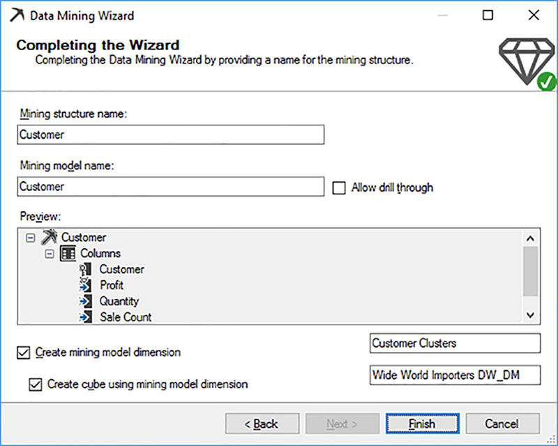
9. Right-click the project in Solution Explorer, and select Deploy to deploy the updates to the SSAS server and process.
10. Double-click the Wide World Importers DW_DM.cube file in Solution Explorer, click the Browser tab in the cube designer, expand the Measures folder, expand the Sale folder, and drag Profit to the query window. Then expand the Customer Clusters folder and then drag MiningDimensionContentNodes to the query window to view the breakdown of sales by cluster. When you use more realistic data than WideWorldImportersDW, more clusters are likely to be available for analysis.
Note Data mining model viewer
To view the characteristics of each cluster, double-click the Customer.dmm file in Solution Explorer and click the Mining Model Viewer tab. Here you can switch between the Cluster Diagram, Cluster Profiles, Cluster Characteristics, and Cluster Discrimination tabs to explore visualizations, statistics, and other information about the clusters created by the data mining algorithm. You are not tested on the use of the data mining model viewer on the exam, but you can learn more about using it in “Browse a Model Using the Microsoft Cluster Viewer” at https://msdn.microsoft.com/en-us/library/ms174801.aspx.
Many-to-many dimension model
The use of a many-to-many dimensional model is necessary when you need to support a more complex type of analysis than we have explored to this point. Traditional analysis is a one-to-many model in which one dimension member can be associated with many fact rows. Put another way, a single fact row is associated with one member in a related dimension. In a many-to-many relationship, a single fact row can be associated with many dimension members.
This type of modeling is common in banking analysis in which a single bank account can be associated with multiple account holders, and therefore a transaction in a fact table has a many-to-many relationship with account holders. The medical industry also often requires many-to-many modeling. As an example, a patient can have multiple diagnoses, so an event such as a hospital stay can be associated with multiple members in a diagnosis dimension.
As a result of implementing this type of model, you can roll up aggregated values within a dimension by different members without overcounting values. Let’s say in a simple cube you have a bank account with two account holders and the account has a $100 balance. If you query balances for all account holders, SSAS lists each account holder separately with the $100 balance, but the aggregate value for all account holders is $100. SSAS knows how to associate the fact rows individually to each dimension member, but also correctly computes the aggregate values for the dimension.
Before you can implement a many-to-many dimension model in SSAS, you need to structure your source tables or DSV appropriately. Nothing in the WideWorldImportersDW source tables lends itself to this type of modeling, so let’s set up a simple scenario in which a new dimension contains sales reasons. Sales reasons describe why a customer made a purchase and are captured in a survey conducted at the time of the purchase. Any sale transaction can be associated with zero to many sales reasons. To model this scenario, you need to add a new Sales Reason dimension and a Sales Reason Bridge to associate sales transactions from the Sale table to the sales reasons in the new dimension, as shown in Figure 1-37.

To set up this scenario in the current project, perform the following steps:
1. Create a named query as a source for the Sales Reason dimension. To do this, double-click Wide World Importers DW.dsv in Solution Explorer to open the DSV designer.
2. In the diagram pane, right-click anywhere in the diagram pane, and select New Named Query.
3. In the Create Named Query dialog box, type Sales Reason in the Name box, replace the SELECT statement with the statement shown in Listing 1-5, and then click OK.
LISTING 1-5 Named query statement to create Sales Reason dimension
SELECT
1 AS SalesReasonKey, 'Value' AS SalesReason
UNION
SELECT
2 AS SalesReasonKey, 'Manufacturer' AS SalesReason
UNION
SELECT
3 AS SalesReasonKey, 'Sales Person' AS SalesReason;
4. Right-click SalesReasonKey in the diagram, and select Select Logical Primary Key.
5. Now create a bridge table to define the relationship between the fact table and the new dimension. In the diagram pane of the DSV, right-click anywhere, and select New Named Query.
6. In the Create Named Query dialog box, type Sales Reason Bridge in the Name box, replace the SELECT statement with the statement shown in Listing 1-6, and then click OK.
LISTING 1-6 Named query statement to create Sales Reason fact bridge
SELECT
CAST(1 AS bigint) AS [Sale Key],
1 AS SalesReasonKey
UNION
SELECT
CAST(1 AS bigint) AS [Sale Key],
2 AS SalesReasonKey
UNION
SELECT
CAST(1 AS bigint) AS [Sale Key],
3 AS SalesReasonKey
UNION
SELECT
CAST(2 AS bigint) AS [Sale Key],
1 AS SalesReasonKey;
7. Select the Sale Key column in the Sales Reason Bridge table and drag it to the Sale key column in the Sale table to define a new relationship.
8. Repeat the previous step to create a relationship between SalesReasonKey in the Sales Reason Bridge table and the SalesReasonKey column in the Sales Reason table.
9. Create the Sales Reason dimension in the project by following the steps described in the “Develop dimension” section earlier in this chapter, using Sales Reason as the Main Table and setting Sales Reason Key as the Key Column and Sales Reason as the Name Column. Click Next twice, and click Finish.
10. Rename the Sales Reason Key attribute to Sales Reason.
11. Double-click Wide World Importers DW.cube in Solution Explorer to open the cube designer.
12. Right-click in the Dimension pane on the Cube Structure page, select Add Cube Dimension, select Sales Reason, and click OK.
13. Right-click the Measures pane, select New Measure Group, and select Sales Reason Bridge to add the bridge table to the cube.
14. Expand the Sales Reason Bridge folder in the Measures pane, select Sales Reason Bridge Count, and then, in Properties window, select False in the Visible drop-down list.
15. Open the Dimension Usage page of the cube designer. Notice the Invoice and Sales Reason dimensions have a regular relationship with the Sales Reason Bridge measure group.
16. To set up the many-to-many relationship, click the intersection between Sales Reason and Sale, click the ellipsis button, select Many-To-Many in the Select Relationship Type drop-down list, select Sales Reason Bridge in the Intermediate Measure Group drop-down list, as shown in Figure 1-38, and click OK.

17. Deploy the project, and then open the Browser page of the cube designer, click Reconnect in the toolbar.
18. On the Cube menu, select Analyze In Excel. Click Enable in the Microsoft Security Notice message box.
19. In the PivotTable Fields list, drag the Invoices check box to the Filters pane below the list.
20. In the pivot table, open the drop-down list, select the Select Multiple Items check box, clear the All check box, expand All, and select the 1 and 2 check boxes.
21. In the PivotTable Fields list, select the Sale Count check box, and notice the pivot table displays a total of 3.
22. In the PivotTable Fields list, select the Invoice check box and notice there are two invoices, 1 and 2. Invoice 1 has a sale count of 1 and Invoice 2 has a sale count of 2.
23. Now select Sales Reason in the PivotTable Fields list. A second level is added to the pivot table in which there are three sales reasons for Invoice 1, each with a sale count of 1: Value, Manufacturer, and Sales Person. Invoice 2 has one sales reason, Value, with a sale count of 1. Notice the total remains 3 in spite of the four instances of sales reasons in the pivot table having a sale count of 1. The sale counts are not overcounted even when a many-to-many relationship is present in the query’s dimensions.
Need More Review? Many-to-many dimensional modeling
You can find a thorough coverage of the challenges with many-to-many dimensional modeling and potential solutions in “Many to Many Revolution 2.0” by Marco Russo and Alberto Ferrari available for download from http://www.sqlbi.com/articles/many2many/.
Slowly changing dimension model
As explained in the “Source table design” section in Skill 1.1, “Create a multidimensional database by using Microsoft SQL Server Analysis Services (SSAS),” there are two types of SCD tables that you can design and then add to your DSV—Type 1 for which you do not track historical changes, and Type 2 for which you track historical changes. When you use the Type 1 SCD design, you do not need to perform any additional tasks in the DSV or dimension design, although you should be aware of the effect of data changes during processing as explained in Chapter 4, which in turn can influence how you configure attribute relationships as described later in this skill. On the other hand, when you use the Type 2 SCD design, there are some specific tasks you should perform in the dimension design to support the ability to browse both the current version and the historical version of dimension attributes.
The first task is to ensure your Type 2 SCD table design includes columns to support slowly changing dimensions as described in Skill 1.1. That is, you must have a surrogate key, a business key, SCD history columns, and at least one attribute for which values change over time for which you want to preserve history.
The Stock Item table in the Wide World Importers DW DSV meets these criteria; so let’s add it to the project as a slowly changing dimension by following the steps described in the “Develop dimension” section earlier in this chapter and then performing these steps:
1. In the Dimension Wizard, use Stock Item as the Main Table, set Stock Item Key as the Key Column, and set Stock Item as the Name Column.
2. In the Select Dimension Attributes page of the wizard, keep the Stock Item Key check box selected, and then select the WWI Stock Item ID check box to add the business key, the Color check box to add the SCD attribute, and the Size check box to add an unchanging attribute. Then click Next, and click Finish.
3. Your next set of tasks is to change properties for the surrogate key and business key attributes. First, rename the Stock Item Key as Stock Item History, and WWI Stock Item ID as Stock Item.
4. Next, set the NameColumn property for the business key. The NameColumn property is set automatically for the surrogate key by the wizard. In this case, you use the same column to define the Name Column property for the business key. To do this, select Stock Item (the renamed business key attribute) in the Attributes pane of the dimension designer, scroll down to locate the NameColumn property, click the box to the right of the property name, click the ellipsis button that displays, select Stock Item in the Name Column dialog box, and then click OK.
5. Last, add the dimension to a cube. In Solution Explorer, double-click Wide World Importers DW.cube, right-click inside the Dimensions pane on the Cube Structure page of the cube designer, select Add Cube Dimension, select Stock Item, and click OK. The dimension usage is set correctly by default with a regular relationship due to the relationship defined between the Sale fact table and the Stock Item dimension table, so no additional configuration is required.
6. There is no data in the World Wide Importers DW sales to properly illustrate the effect of SCD changes, so execute the statement shown in Listing 1-7 to add a new sale using the surrogate key for a current stock item.
LISTING 1-7 Insert a row into the sales fact table for a current stock item
INSERT INTO [Fact].[Sale]
([City Key],
[Customer Key],
[Bill To Customer Key],
[Stock Item Key],
[Invoice Date Key],
[Delivery Date Key],
[Salesperson Key],
[WWI Invoice ID],
[Description],
[Package],
[Quantity],
[Unit Price],
[Tax Rate],
[Total Excluding Tax],
[Tax Amount],
[Profit],
[Total Including Tax],
[Total Dry Items],
[Total Chiller Items],
[Lineage Key])
VALUES
(0,
0,
0,
604,
'2016-05-31',
'2016-05-31',
0,
70511,
'USB rocket launcher (Gray)',
'Each',
1000,
25,
15,
25000,
3750,
15500,
28750,
1000,
0,
11);
GO
7. Deploy the project to see how the SCD design affects query results. Right-click the project in Solution Explorer, select Deploy, and click Yes to overwrite the database on the server.
8. After deployment is complete, click the Browser page of the cube designer, and click the Reconnect button in the toolbar.
9. Now set up the query. Expand the Measures folder in the metadata pane, expand the Sale folder, and then drag Sale Count to the query window.
10. Next, expand Stock Item in the metadata tree. This top-level Stock Item node represents the dimension as indicated by the icon containing a cube and arrows pointing in three directions. Below this is another Stock Item node, which is an attribute as indicated by the set of blue squares arranged in a rectangular shape.
11. Drag the Stock Item attribute to the query window, and then drag the right edge of the column header to the right to widen the column for better visibility of each stock item’s name, as shown in Figure 1-39. Notice that the current count for USB Rocket Launcher (Gray) is 1079.

FIGURE 1-39 Metadata pane and query window on the Browser page of the cube designer showing sale counts by stock item
12. If you drag the Color attribute into the query window, you see the Sale Count is 1078 for the historical color Gray and 1 for the current color Steel Gray. The Stock Item attribute is an aggregate of all historical information, but you can also view the historical information for the changing attribute Color when you add it to the query.
13. Now drag the Stock Item column header from the query window to the left to remove it from the query, and then drag Stock Item History from the metadata pane to the query window. Drop it to the left of the Color column.
14. Next, filter the query to more easily locate the stock item in the previous query. To do this, select Stock Item in the Dimension drop-down list above the query window, and select Stock Item History in the Hierarchy drop-down list.
15. In the Operator drop-down list, select Begins With. In the Filter Expression box, type USB rocket launcher and press Enter. Then remove the Color column. Now you see two stock items with the same name, as shown in Figure 1-40, because these two dimension members have separate surrogate keys, and each surrogate key appears in one or more rows in the fact table.

FIGURE 1-40 Metadata pane and query window on the Browser page of the cube designer showing sale counts by stock item history
When you include the Color attribute in the query, you can see that each Stock Item History member corresponds to a different color. However, when Color is not included in the query, the appearance of two separate rows in the query results is potentially confusing to business users. For this reason, a common design approach for modeling SCDs is to hide the attribute associated with the surrogate key so that business users cannot accidentally use it in a query when exploring the cube.
16. In this case, you can hide the Stock Item History attribute by returning to the Stock Item dimension designer, selecting Stock Item History in the Attributes pane, and changing the AttributeHierarchyVisible property in the Properties window to False.
Note AttributeHierarchyVisible versus AttributeHierarchyEnabled
On the surface, both the AttributeHierarchyVisible and AttributeHierarchyEnabled appear to have the same behavior because if you change either property to False for an attribute, that attribute is not available to add to a query when browsing the cube. However, under the covers, the behavior is different. SSAS does not allocate dimension storage space to an attribute for which AttributeHierarchyEnabled is False. Instead, the attribute is converted to a member property as described in the “Develop a dimension” section earlier in this chapter. By contrast, dimension storage space is allocated to an attribute with its AttributeHierarchyVisible set to False. When dimension storage space is allocated, dimension processing time is increased.
17. After you deploy the project, you can reconnect to the cube on the Browser page of the cube designer and confirm that the Stock Item History attribute no longer appears in the metadata pane, as shown in Figure 1-41.

FIGURE 1-41 Metadata pane in the Browser page of the cube designer showing the Stock Item dimension’s attributes after hiding the key attribute
Note Consider the impact of SCD modeling on query performance
If you have a large dimension, the modeling approach described here can potentially result in poor query performance. One way to mitigate this potential problem is to add a user-defined hierarchy and configure attribute relationships properly, as described in the “Define attribute relationships” section later in this chapter.
Implement a dimension type
Each dimension has a Type property that is set by default to Regular. In general, when the property is not set to Regular, the Type setting instructs either the SSAS server, the client application, or both the server and client application how to perform certain types of calculations to alleviate the need to create complex calculated members, custom rollup formulas, or MDX scripts. Typically, you must also define a Type property for one or more attributes in the dimension to configure the desired behavior.
You can choose from the following Type values to define the applicable calculation behavior for a dimension:
![]() Accounts Sets specific server-side behaviors for aggregating financial accounts. When you use this dimension type, you must also configure an attribute’s Type property as AccountType for the attribute containing members such as Assets, Liabilities, Revenue, and so on. SSAS uses the account type to determine whether to aggregate values for dates within a calendar or fiscal year for income statement accounts (such as revenue and expenses), or to compute point-in-time values for balance sheet accounts (such as assets and liabilities).
Accounts Sets specific server-side behaviors for aggregating financial accounts. When you use this dimension type, you must also configure an attribute’s Type property as AccountType for the attribute containing members such as Assets, Liabilities, Revenue, and so on. SSAS uses the account type to determine whether to aggregate values for dates within a calendar or fiscal year for income statement accounts (such as revenue and expenses), or to compute point-in-time values for balance sheet accounts (such as assets and liabilities).
Note Financial Account dimension type
There is no financial account data available in the WideWorldImportersDW database to help you explore working with the Accounts type, but you should be familiar with the concepts for the exam. You can learn more about working with this type of dimension by reading “Create a Finance account of parent-child type Dimension” at https://technet.microsoft.com/en-us/library/ms174609(v=sql.130).aspx.
![]() BillOfMaterials (BOM) Organizes a dimension by attributes that define how parts comprise a unit and requires you to define attributes such as organizational unit, BOM resource, and quantitative. A client application controls how this information drives dimension behavior.
BillOfMaterials (BOM) Organizes a dimension by attributes that define how parts comprise a unit and requires you to define attributes such as organizational unit, BOM resource, and quantitative. A client application controls how this information drives dimension behavior.
![]() Channel Represents channel information and requires a client application to determine how this information is used.
Channel Represents channel information and requires a client application to determine how this information is used.
![]() Currency Defines the currency conversion behavior for a dimension.
Currency Defines the currency conversion behavior for a dimension.
The WideWorldImportersDW database does not include currency conversion data, but you do not need to know how to configure currency conversion dimensions for the exam. Nonetheless, if you want to learn more, see “Create a Currency type Dimension” at https://technet.microsoft.com/en-us/library/ms175413(v=sql.130).aspx. Boyan Penev has a blog post, “A Guide to Currency Conversions in SSAS”, that provides a comprehensive review of available resources for configuring a currency dimension and illustrates a solution for handling currency conversion that you should review at http://www.bp-msbi.com/2010/10/a-guide-to-currency-conversions-in-ssas/. Another resource that spells out step by step how to configure currency conversion is provided by Hennie de Nooijer in “SSAS: Multicurrency Problem (Part I)” at http://bifuture.blogspot.com/2014/09/ssas-multicurrency-problem-part-i.html.
![]() Customers Organizes attributes for information about customers, such as name, address, demographic details, and more. You must use a client application that supports this dimension type to see behavior change.
Customers Organizes attributes for information about customers, such as name, address, demographic details, and more. You must use a client application that supports this dimension type to see behavior change.
![]() Geography Requires a client application to define dimension behavior, such as displaying aggregated data projected onto a geographic visualization. This dimension type contains attributes for geographical areas, such as postal code, city, or country.
Geography Requires a client application to define dimension behavior, such as displaying aggregated data projected onto a geographic visualization. This dimension type contains attributes for geographical areas, such as postal code, city, or country.
![]() Time Sets the behavior for calculations that are dependent on time. By setting the Type property appropriately for each attribute, you identify the attributes containing years, quarters, months, days, and so on.
Time Sets the behavior for calculations that are dependent on time. By setting the Type property appropriately for each attribute, you identify the attributes containing years, quarters, months, days, and so on.
![]() Organization Defines a dimension containing attributes about subsidiary organizations, ownership percentages, and voting rights percentages. A client application controls how this information affects calculations or dimension behavior in an application.
Organization Defines a dimension containing attributes about subsidiary organizations, ownership percentages, and voting rights percentages. A client application controls how this information affects calculations or dimension behavior in an application.
![]() Products Organizes a dimension by attributes describing characteristics of parts, such as color, size, category, and so on. This dimension type requires a client application to use this information.
Products Organizes a dimension by attributes describing characteristics of parts, such as color, size, category, and so on. This dimension type requires a client application to use this information.
![]() Promotion Describes a dimension containing information about marketing promotions. This information is used only within a client application that supports this dimension type.
Promotion Describes a dimension containing information about marketing promotions. This information is used only within a client application that supports this dimension type.
![]() Quantitative Requires a client application that can use attributes containing quantitative values.
Quantitative Requires a client application that can use attributes containing quantitative values.
![]() Rates Defines the dimension containing currency rate information that the SSAS server uses for currency conversions in conjunction with the Currency dimension type. Refer to the additional resource recommended for the Currency dimension type to learn how to use this dimension type properly.
Rates Defines the dimension containing currency rate information that the SSAS server uses for currency conversions in conjunction with the Currency dimension type. Refer to the additional resource recommended for the Currency dimension type to learn how to use this dimension type properly.
![]() Scenario Identifies a dimension containing attributes to define a scenario, such as budgeting or forecasting, and a version.
Scenario Identifies a dimension containing attributes to define a scenario, such as budgeting or forecasting, and a version.
![]() Utility Flags a dimension for a purpose to be defined by a client application.
Utility Flags a dimension for a purpose to be defined by a client application.
The most common implementation of a dimension type other than the default of Regular is to set a Date dimension as a Time dimension type. Let’s add some additional attributes to this dimension and then explore the additional configuration required in the dimension to achieve the desired results.
To set the Type property of the Date dimension, double-click the Date.dim file in Solution Explorer, click the dimension name (the top level node) in the Attributes pane of the dimension designer, and then select Time in the Type drop-down list in the Properties window. You must also configure each attribute with the applicable type by selecting the attribute in the Attributes pane, and selecting the correct value, shown in Table 1-3, in the Type drop-down list. When you navigate through the list of values in the Type drop-down list, you must expand nodes within a type category to find the type you want. For example, you can expand Date, and then Calendar to find Months (shown in the table as Date/Calendar/Months), or expand ISO to find Iso8601WeekOfYear. In addition, change the Name property of each attribute if it is included in Table 1-3.

Exam Tip
Each specific property setting requires different additional configuration settings and results in different behaviors. If the dimension type is used only by client applications, you must refer the application documentation to learn how to configure the dimension and its attributes properly. For this reason, the exam does not test your knowledge about those dimension types. However, you should know how to work with the Time, Account, Currency, and Rate dimension types.
Define attribute relationships
A best practice in multidimensional database development is the addition of user-defined hierarchies. A user-defined hierarchy (in which the user is you, as the developer, and not the business user who queries the cube) is a pre-defined navigation path for moving from summary to detail information. For example, you use a hierarchy to make it easier to view sales by year, then by month, and then by day, as shown in Figure 1-42.

Each level of a hierarchy corresponds to a separate attribute in the dimension. For example, in the hierarchy shown in Figure 1-42, the top level of the hierarchy is the Calendar Year attribute, the middle level is the Calendar Month attribute, and the bottom level is the Date attribute.
After creating a hierarchy, you might also need to define attribute relationships between each level in the hierarchy. Attribute relationships determine how SSAS calculates aggregate values within a cube and how it stores data on disk. For this reason, the presence or absence of attribute relationships potentially affects query performance.
Before you can work with attribute relationships, you must first create a hierarchy. To do this for the Date dimension, perform the following steps:
1. Open the dimension designer for Date, drag the Calendar Year attribute from the Attributes pane to the Hierarchies pane of the designer. When you drop it, a new hierarchy is created.
2. You can then add levels to the new hierarchy by dragging the Calendar Month attribute into the hierarchy object below the Calendar Year attribute, and then repeating this process with the Date attribute.
3. Right-click the Hierarchy caption for the new hierarchy in the Hierarchies pane, select Rename, and type Calendar to rename it.
You can create as many hierarchies as you like. Technically speaking, you can create only 2,147,483,647 user-defined hierarchies, but you probably do not need that many!
4. For now, create another hierarchy renamed as ISO Calendar by using the Calendar Year, ISO Week Number, and Date attributes, as shown in Figure 1-43.
Important Hierarchy name must be unique
The hierarchy name must be unique within the dimension, not only with regard to other hierarchies but it also cannot conflict with attribute names in the same dimension.

Notice the warning icon and best practice warning indicated by the wavy underscore below each hierarchy name to indicate a potential problem. If you hover the cursor over each warning, the following message displays: “Attribute relationships do not exist between one or more levels of this hierarchy. This may result in decreased query performance.” This is a very common warning.
Behind the scenes, SSAS sets up attribute relationships between the hierarchy levels and the key attribute where possible. To review the current definition for attribute relationships, click the Attribute Relationships tab in the dimension designer. As shown in Figure 1-44, the relationships between the key attribute, Date, and the attributes on the levels of each hierarchy are visible as arrows connecting Date to ISO Week Number, Calendar Year, and Calendar Month.

The hierarchy warnings on the Dimension Structure page displays because Calendar Year is part of both hierarchies, but does not connect directly to the attribute in the child level in either hierarchy. The dimension can process successfully in this state, but the warning message alerts you that there could be an adverse impact on query performance. With this database, the volume of data is too small for you to notice slow query performance. However, once you start working with fact tables having millions or billions of rows, the performance problem becomes more noticeable.
Before you decide whether you need to fix this particular warning, you must know what type of hierarchy you have created. A natural hierarchy is a hierarchy for which each attribute has a one-to-many relationship between dimension members on a parent level and dimension members on a child level, as shown in Figure 1-45. In the Date dimension, the Calendar hierarchy is a natural hierarchy because each Calendar Month member corresponds to one, and only one, member on the Calendar Year level.

Note Natural hierarchy attribute relationships benefit query performance
The primary reason that natural hierarchy attribute relationships improve query performance is the materialization of hierarchical data on disk for faster retrieval. At query time, SSAS can navigate specific structures built for hierarchical data storage to find specific combinations, such as ISO Week Number 1 for CY2013, quickly rather than starting with a key attribute such as 2013-01-01 and working through the attribute structures to locate the related ISO Week Number and Calendar Year. Also, SSAS maintains indexes to know which combinations exist or not and thereby retrieve data more efficiently. For example, by scanning the index, SSAS knows that 2013-01-07 is not associated with ISO Week Number 1, and can eliminate the combination when constructing query results that require a cross join of Date and ISO Week Number values.
Admittedly, in a relatively small dimension such as Date, the difference in query performance with or without a natural hierarchy is negligible. However, in large dimensions, the existence of accurate attribute relationships has a measurable impact on performance.
Furthermore, when attribute relationships exist, SSAS can design and store aggregations that also contribute to faster queries. You learn how to work with aggregations to improve query performance in Chapter 4.
By contrast, an unnatural hierarchy is one for which there is the potential to have a many-to-many relationship between members on a parent and child levels. To create an unnatural hierarchy, open the Stock Item dimension designer and create a hierarchy named Color-Size with Color as the top level, and Size as the bottom level. Figure 1-46 illustrates the partial results of these attribute combinations in a hierarchy.

You use an unnatural hierarchy to enable users to report on combinations of dimension members that are not hierarchical. That way, you can build into your multidimensional database the ability to produce the same result as a relational query that aggregates the quantity sold and group the aggregate value by two different, non-hierarchical columns, as shown in Listing 1-8.
LISTING 1-8 Retrieve aggregate results from a relational database by using a GROUP BY clause
USE WideWorldImportersDW;
GO
SELECT
Color,
Size,
SUM(Quantity) AS QuantitySold
FROM Fact.Sale s
INNER JOIN Dimension.[Stock Item] si
ON s.[Stock Item Key] = si.[Stock Item Key]
GROUP BY
Color,
Size;
If you review the attribute relationships of an unnatural hierarchy, as shown in Figure 1-47, you can see there is no arrow connecting the attributes of the hierarchy’s level. Instead, each level’s attribute relates back to the key attribute, Stock Item History. In the case of an unnatural hierarchy, this lack of attribute relationships between the hierarchy’s attributes is appropriate.

Whenever you see the warning about non-existent attribute relationships between hierarchy levels, you should evaluate whether the hierarchy is natural or unnatural. If it is natural, you must fix the attribute relationships, but you can ignore the warning if the hierarchy is unnatural. However, you should test whether the performance of queries using the unnatural hierarchy is acceptable. If it is not, consider modify the dimension structure to transform the unnatural hierarchy into a natural hierarchy.
Let’s say that you want to optimize the natural hierarchies, Calendar and ISO Calendar, by fixing the attribute relationships. To do this, perform the following steps:
1. Open the Attribute Relationships page of the Date dimension designer. Then drag the ISO Week Number object in the diagram to the Calendar Year object and drag the Calendar Month object to the Calendar Year object to create the relationships shown in Figure 1-48.

These adjustments clear the warnings from the Dimension Structure page of the dimension designer. However, a new problem is introduced because the data is not currently structured to support a natural hierarchy for ISO Calendar.
2. To see the results caused by this problem, deploy the project. Deployment fails due to the following warning that displays in the Output window: “Errors in the OLAP storage engine: A duplicate attribute key has been found when processing: Table: ‘Dimension_Date’, Column: ‘ISO_x0020_Week_x0020_Number’, Value: ‘15’. The attribute is ‘ISO Week Number’.”
3. The best way to see the problem with the duplicate attribute key is to process the Date dimension manually so that you can extract the SQL query that SSAS generates, and review the query results in SSMS. First, right-click Date.dim in Solution Explorer, select Process, select Process Full in the Process Options drop-down list if it is not already selected, and click Run.
4. In the Process Progress dialog box, expand Processing Dimension ‘Date’ Completed, expand Processing Dimension Attribute ‘ISO Week Number’ Completed, expand SQL Queries 1, click the SELECT statement, and click View Details to see the full query, as shown in Figure 1-49.

5. Highlight the entire SELECT statement, and press CTRL+C to copy the statement to the clipboard. Click Close three times to close all open dialog boxes.
6. Next, open SSMS, connect to the database engine hosting the WideWorldImportersDW database, click the New Query button in the toolbar, select WideWorldImportersDW in the Available Databases drop-down list in the toolbar, paste the statement into the Query window. Modify the query to add an ORDER BY clause as shown in Listing 1-9, and click Execute.
LISTING 1-9 Review results of query generated by SSAS for populating the ISO Week Number attribute
SELECT
DISTINCT
[Dimension_Date].[ISO Week Number] AS
[Dimension_DateISO_x0020_Week_x0020_Number0_0],
[Dimension_Date].[Calendar Year Label] AS
[Dimension_DateCalendar_x0020_Year_x0020_Label0_1]
FROM [Dimension].[Date] AS [Dimension_Date]
ORDER BY [Dimension_Date].[ISO Week Number];
As you can see by the partial results shown in Figure 1-50, each ISO Week Number value in the first column corresponds to four different Calendar Year values in the second column. Because of the attribute relationship that exists between ISO Week Number and Calendar Year, there can be only one Calendar Year parent member for each ISO Week Number child member. Otherwise, dimension processing fails.

An easy way to fix this problem is to modify the key column for the ISO Week Number attribute to create a unique value for each ISO Week Number-Calendar Year combination. To do this, perform the following steps:
1. Open the Dimension Structure tab of the dimension designer, select ISO Week Number in the Attributes pane, click the KeyColumns box in the Properties window, and then click the ellipsis button.
2. In the Key Columns dialog box, click Calendar Year in the Available Columns List, click the > button, select Calendar Year in the Key Columns list, click the Up button to place Calendar Year ahead of ISO Week Number in the list, and click OK.
3. Next, click the NameColumn box in the Properties window, click the ellipsis button, select ISO Week Number, and click OK.
4. Last, deploy the project to update the multidimensional database on the server with your changes.
Important Changing a dimension impacts mining structures
If you created the Customer mining structure in the “Data mining dimension model” section earlier in this chapter, the change to the ISO Week Number key columns invalidates the Customer mining structure. Because you no longer use this mining structure and the related dimension and cube in the project used in this chapter, you can safely delete these three files. Right-click Wide World Importers DW_DM.cube in Solution Explorer, select Delete, and click OK to confirm. Repeat these steps to remove Customer Clusters.dim and Customer.dmm from the project. You can then successfully deploy the project to update the Date dimension on the server.
Like attributes, attribute relationships have properties. You can select an arrow in the diagram or select a relationship in the Attribute Relationships pane to view the following properties in the Properties window.
![]() RelationshipType Determines how SSAS manages changes to the key column for a related attribute. The default value is Flexible, which allows changes to occur without requiring you to perform a full process of the dimension. (The implications of relationship types on dimension processing is described more fully in Chapter 4.) For example, if you expect Color to change frequently for a stock item, you can set the relationship between Stock Item History and Color to Flexible.
RelationshipType Determines how SSAS manages changes to the key column for a related attribute. The default value is Flexible, which allows changes to occur without requiring you to perform a full process of the dimension. (The implications of relationship types on dimension processing is described more fully in Chapter 4.) For example, if you expect Color to change frequently for a stock item, you can set the relationship between Stock Item History and Color to Flexible.
Your other option is to set this property to Rigid. In that case, any change in the relationship between an attribute and a related attribute requires you to fully process the dimension. You use this option when you expect the relationships between attributes rarely or never to change, such as the assignment of a date to a month, or when you expect values to rarely change. The date 2013-01-01 always remains a child of CY2013-Jan and never gets reassigned to CY2013.
![]() Attribute Specifies the attribute on which the attribute relationship is based. In other words, this property defines the parent attribute in the relationship.
Attribute Specifies the attribute on which the attribute relationship is based. In other words, this property defines the parent attribute in the relationship.
![]() Cardinality Describes the relationship has a many-to-one or one-to-one relationship between the child attribute and the parent attribute. The default is Many to indicate a many-to-one relationship, such as exists between Date and Calendar Month in which there are many dates related to a single month. This is the most common scenario that you find in attribute relationships.
Cardinality Describes the relationship has a many-to-one or one-to-one relationship between the child attribute and the parent attribute. The default is Many to indicate a many-to-one relationship, such as exists between Date and Calendar Month in which there are many dates related to a single month. This is the most common scenario that you find in attribute relationships.
You change the value to One when you want to specify a one-to-one relationship. For example, if you had an attribute for telephone number in the Customer dimension, you would define the relationship between that attribute and the Customer attribute by setting the Cardinality property to one.
![]() Name Provides a unique name for the relationship. This value defaults to the name of the parent attribute.
Name Provides a unique name for the relationship. This value defaults to the name of the parent attribute.
![]() Visible Determines whether a client application can access the parent attribute as a member property in an MDX query. Working with member properties is described in more detail in Chapter 3.
Visible Determines whether a client application can access the parent attribute as a member property in an MDX query. Working with member properties is described in more detail in Chapter 3.
Need More Review? Attribute relationships and performance tuning
Although written for SQL Server 2012 and 2014, you can find performance tuning recommendations related to attribute relationships in “Analysis Services MOLAP Performance Guide for SQL Server 2012 and 2014” by Karan Gulati and John Burchel. This whitepaper is available for download at https://msdn.microsoft.com/en-us/library/dn749781.aspx. The architectural changes to the multidimensional database engine in SQL Server 2016 do not change the recommendations in this whitepaper for attribute relationships.
Skill 1.3: Implement measures and measure groups in a cube
Often you continue adding measures and measure groups to a cube after using the Cube Wizard because it is easier to develop and test a cube incrementally rather than trying to add everything at once in the wizard. Another post-wizard task is to configure various properties for measures and measure groups in your cube to control behavior. Among other reasons, you can use properties to control how values aggregate from detail to summary levels or to apply a format string for better legibility.
Design and implement measures, measure groups, granularity, calculated measures, and aggregate functions
The cube designer provides a lot of functionality for developing your cube beyond the basic configuration defined by using the Cube Wizard. You can use it to add new measures and configure properties for those measures in addition to bringing in multiple measures in a bulk for a new measure group. You can also use it to adjust the granularity of relationships between measure groups and dimensions. Not only can you define measures from which values are retrieved from a source fact table, but you can also define calculated measures, which are measures derived by defining expressions that operate on fact-sourced measures. Last, an important step in cube development is ensuring that SSAS applies the appropriate aggregate function to each measure, which you also configure in the cube designer.
Measures
The “Develop a cube” section of Skill 1.1 described how to add measures to a cube in bulk by using the Cube Wizard. You can also add measures manually to an existing cube or change properties for measures by using the cube designer.
To add a new measure to an existing cube, perform the following steps:
1. Double-click the Wide World Importers DW.cube file in Solution Explorer, right-click the Sale measure group in the Measures pane on the Cube Structure page of the cube designer, and select New Measure.
In the current cube, all numeric columns that represent measures already exist in the cube, but if you had omitted a measure based on one of these columns when using the Cube Wizard, you could select it in the Source Columns list in the New Measure dialog box, and add it to your cube.
2. Another option is to create a distinct count measure based on a key column in the fact table. For example, let’s say that you want to include the ability to show the distinct count of stock items sold to each customer or sold on a given day. To do this, select the Show All Columns check box in the New Measure dialog box, select Distinct Count in the Usage drop-down list, select Stock Item Key in the Source Column list, as shown in Figure 1-51, and click OK.

Rather than appearing in the Sales measure group, Stock Item Key Distinct Count appears in a newly added measure group named Sale 1 because distinct count measures are managed differently from other measures by SSAS. Because the calculation of a distinct count value at query time is expensive for SSAS to perform, SSAS places each distinct count measure into its own measure group. You can rename the measure group by right-clicking it and typing a new name.
After you create a measure, or after adding several measures by using the Cube Wizard, you should review measure properties to ensure that each measure behaves as expected when business users browse the cube. You can review a measure’s properties by selecting the measure in the Measures pane of the cube designer, and then scrolling through the Properties window. Each measure has the following set of properties that you can configure:
![]() AggregateFunction Determines how SSAS aggregates detail rows from the fact table to summary values. The most commonly used AggregateFunction property is Sum. The other AggregateFunction values are explained later in this section.
AggregateFunction Determines how SSAS aggregates detail rows from the fact table to summary values. The most commonly used AggregateFunction property is Sum. The other AggregateFunction values are explained later in this section.
![]() DataType Inherits from the data type for the measure column in the source fact table.
DataType Inherits from the data type for the measure column in the source fact table.
![]() DisplayFolder Specifies the folder in which to display the measure in the client application. You type in the name of a new folder or select the name of an existing folder in the property’s drop-down list. Using a display folder is helpful for logically organizing measures when the measure group contains a lot of measures.
DisplayFolder Specifies the folder in which to display the measure in the client application. You type in the name of a new folder or select the name of an existing folder in the property’s drop-down list. Using a display folder is helpful for logically organizing measures when the measure group contains a lot of measures.
![]() MeasureExpression Defines an MDX expression that resolves the value for a measure at the leaf level before aggregation. A common reason to implement a measure expression is to multiply a sales value by an exchange rate prior to summing up the sales values.
MeasureExpression Defines an MDX expression that resolves the value for a measure at the leaf level before aggregation. A common reason to implement a measure expression is to multiply a sales value by an exchange rate prior to summing up the sales values.
![]() Visible Determines whether the client application displays the measure. If you change this property to False, you can still reference the measure in MDX expressions, which is useful when the base measure is not required for analysis.
Visible Determines whether the client application displays the measure. If you change this property to False, you can still reference the measure in MDX expressions, which is useful when the base measure is not required for analysis.
![]() Description Allows you to provide additional information about a measure for display in a client application.
Description Allows you to provide additional information about a measure for display in a client application.
![]() FormatString You can select a format string from a list of possible formats, such as Percent or Currency, or type in a user-defined format, such as #,# to display an integer value with a thousands separator. You can use any valid Microsoft Visual Basic custom format for numeric values as a format string.
FormatString You can select a format string from a list of possible formats, such as Percent or Currency, or type in a user-defined format, such as #,# to display an integer value with a thousands separator. You can use any valid Microsoft Visual Basic custom format for numeric values as a format string.
![]() Name Provides a name for display in client applications or for reference in MDX expressions.
Name Provides a name for display in client applications or for reference in MDX expressions.
![]() Source Binds the measure to a specific table and column in the DSV.
Source Binds the measure to a specific table and column in the DSV.
Currently, when you browse the cube, the default properties for each measure are in effect. If you browse the cube in the cube designer, you cannot see formatting. Although no formatting is set yet, you can set up a baseline query by using Excel to browse the cube. To do this, perform the following steps:
1. Open the Browser tab of the cube designer, and then select Analyze In Excel on the Cube menu.
2. Click Enable in the Microsoft Security Notice message box.
3. Next, in the PivotTable Fields list, select the following measures: Profit, Quantity, Sale Count, Tax Rate, Total Excluding Tax, and Unit Price. Scroll down in the PivotTable Fields List to locate and select the Buying Group check box in the Customer dimension.
The results of these selections display in a pivot table, as shown in Figure 1-52. Notice none of these values are formatted for better legibility and currently you can sum the values in each row of a column to produce the Grand Total value in the bottom row.

The three most common changes that are necessary to produce desired results in a cube are to change the AggregateFunction, FormatString, and Name properties of a measure. The AggregateFunction property affects the totals that appear for dimension members in the query as well as the grand total. The FormatString property makes it easier to view the individual values in the query results, whereas the Name property should be a user-friendly name that clearly communicates what the value represents using terms that business users recognize.
To observe the effect of changing the properties of these measures, return to the Cube Structure page of the cube designer, and update the property values as shown for each measure listed in Table 1-4.

Deploy the project, and then switch to Excel. On the PivotTable Analyze tab of the ribbon, click Refresh to update the pivot table with the cube changes. Notice the new formatting of some measures, the missing values for other measures, and missing measures, as shown in Figure 1-53.

Each measure that you renamed no longer appears in the pivot table and must be added back again manually. Add Sales Amount With Tax and Sales Amount Without Tax to the pivot table, and then add Tax Amount so that you can validate the Sales Amount With Tax value in a row by highlighting the Sales Amount Without Tax and Tax Amount columns in the same row, and checking the Sum in the status bar at the bottom of the window, as shown in Figure 1-54.

FIGURE 1-54 Validation of Sales Amount With Tax values by summing Sales Amount Without Tax and Tax Amount
All measures that display with values in the pivot table have the AggregateFunction value set to Sum. These values reflect the sum of all rows in the fact table for the column associated with the respective measure with a grouping by Buying Group. After the AggregateFunction property for Tax Rate and Unit Price is changed to None, the values in the pivot table for those measures no longer display for those measures because SSAS skips the aggregation step when retrieving results for the query. Those values at the row level are still accessible to SSAS for MDX calculations when requested, but summing the tax rate or the unit price for a sale is meaningless for analyzing sales. You can view the values for these two measures at the detail level by double-clicking a cell, such as E2, to open a new Excel sheet that displays the row-level detail in the fact table for the selected cell, as shown in Figure 1-55 in which some columns and rows have been hidden to focus on the columns of interest.
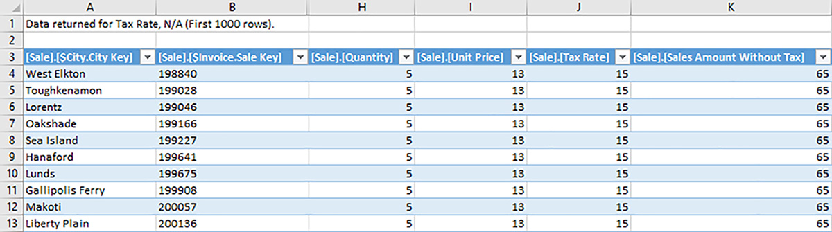
If you switch back to the original sheet containing the pivot table, remove all measures except Sale Count by dragging each measure individually out of the Values pane at the bottom of the PivotTables Fields List. In addition, remove Buying Group from the Rows pane. Then select the Stock Item Distinct Count measure and State Province (from the City dimension) to add them to the pivot table, a portion of which is shown in Figure 1-56.

FIGURE 1-56 A pivot table showing a standard measure, Sale Count, and a distinct count measure, Stock Item Distinct Count
Here you can see the number of sales transactions as the Sale Count value, which counts each row in the fact table and sums it by State Province. However, the Stock Item Distinct Count reflects the distinct count of stock items sold to customers in a specific State Province. If you scroll to the bottom of the pivot table to locate the Grand Total, you find the Sale Count Grand Total is 228,266 and the Stock Item Distinct Count Grand Total is 228. That means there are a total of 228.266 rows in the fact table, but 228 distinct stock item keys in the same table.
Most of the time, measures are additive. That is, regardless of which dimension you include in the query with the measure, the aggregation of the measure by any of the dimension’s attributes is a value that accurately adds up. AggregateFunction property values like Sum or Count are additive measures. You can also define nonadditive measures semiadditive measures as described in more detail in the “Aggregate functions” and “Define semi-additive behavior” sections of this chapter.
Measure groups
Remember from Skill 1.1 that a measure group is a collection of measures that come from the same fact table. A cube can contain multiple measure groups. Ideally, these measure groups share one or more dimensions in common to facilitate analysis and reduce the potential of confusing users. If there are no overlapping dimension, consider creating separate cubes for each measure group.
Before you can add a measure group to a cube, a corresponding table must exist in the DSV. To review how to add a measure group (and later how to work with semi-additive measures), let’s add another fact table to the DSV by performing the following steps:
1. Double-click Wide World Importers DW.dsv in Solution Explorer.
2. Right-click anywhere in the diagram pane of the DSV designer, select Add/Remove Tables, select Stock Holding (Fact) in the Available Objects list, click the > button, and then click OK. The table is added to the DSV with a primary key defined as Stock Holding Key and a relationship added between the Stock Holding table, and the Stock Item table based on the Stock Item Key column.
The Stock Holding table is similar to an inventory table that shows a quantity for each stock item among other information. However, a typical inventory table also includes a date column to show the quantity of each stock item on different dates. Inventory can be tracked yearly, quarterly, monthly, or even daily, depending on business requirements. To better explore semi-additive behavior later in this chapter, you can replace the Stock Holding table with a named query that simulates changes in inventory over time by performing the following steps:
1. Right-click the Stock Holding table in the diagram, point to Replace Table, and select With New Named Query.
2. Replace the SELECT statement in the Create Named Query dialog box with the statement shown in Listing 1-10.
LISTING 1-10 Named query to simulate changes in stock item inventory over time
SELECT
CONVERT(date, '2013-01-01') as DateKey,
[Stock Item Key],
[Quantity On Hand],
[Bin Location],
[Reorder Level],
[Target Stock Level]
FROM
Fact.[Stock Holding]
UNION ALL
SELECT
CONVERT(date, '2013-06-01') as DateKey,
[Stock Item Key],
[Quantity On Hand] - [Stock Item Key] AS [Quantity On Hand],
[Bin Location],
[Reorder Level],
[Target Stock Level]
FROM
Fact.[Stock Holding] AS t;
A surrogate key column is not necessary in a fact table, so the named query eliminates that column along with other extraneous columns so that the results of the named query are simplified as much as possible. In addition, an arbitrary date column is added and a new value is computed for the quantity on hand for the second time period to force a difference in inventory between time periods.
3. Before clicking OK, be sure to type Stock Holding in the Name box at the top of the dialog box if it is not currently correctly named.
4. Press CTRL+S to save the DSV with the new named query.
5. Create a relationship between the Stock Holding and Date tables. Select DateKey in the Stock Holding named query diagram and drag it to the Date column in the Date table.
6. Now you are ready to use the new named query as a new measure group. Double-click the Wide World Importers DW.cube file in Solution Explorer, right-click in the Measures pane of the cube designer, and select New Measure Group. In the New Measure Group dialog box, select Stock Holding, and click OK.
7. In the Measures pane, expand the Stock Holding measure group to review the added measures: Quantity On Hand, Reorder Level, Target Stock Level, and Stock Holding Count.
All numeric columns that are not used in relationships in the DSV are assumed to be measures and added as a group when you create the new measure group. If you do not want to include a measure, such as Stock Holding Count, right-click the measure in the Measures pane, select Delete, and then click OK to confirm the deletion.
8. Set the FormatString property for each of the remaining three measures to #,#.
Each measure group has many different properties available to configure. For the most part, you can keep the default values. Chapter 4 explains more about the properties that affect aggregation design, file placement, and partition processing. For now, let’s consider only the following properties:
![]() IgnoreUnrelatedDimension Determines whether SSAS displays a top-level aggregation value for all members in an unrelated dimension, as shown in Figure 1-57. The default is True.
IgnoreUnrelatedDimension Determines whether SSAS displays a top-level aggregation value for all members in an unrelated dimension, as shown in Figure 1-57. The default is True.

![]() Name Provides a name for display in client applications or for reference in MDX expressions. You can rename a measure group at any time. For example, consider changing the Sale 1 measure group name to Stock Item Sales Distinct Count.
Name Provides a name for display in client applications or for reference in MDX expressions. You can rename a measure group at any time. For example, consider changing the Sale 1 measure group name to Stock Item Sales Distinct Count.
9. On the Dimension Usage page, select the Stock Holding measure group, and then, in the Properties window, change the IgnoreUnrelatedDimension property’s value to False.
10. Deploy the project, open the Browser page of the cube designer, click Reconnect, and set up a query to view Quantity On Hand by Buying Group.
The following message displays: No Rows Found. Click To Execute The Query. Because no relationship exists between the measure and the dimension, and the IgnoreUnrelatedDimension property is False, SSAS has no results to display in the query.
Important Remote linked measure groups deprecated in SQL Server 2016
A linked measure group is a measure group that is created in one database and referenced in one or more separate databases as a method of reusing a common design. For performance reasons, Microsoft recommends that both databases reside on the same server. Linking to a measure group on a remote server is deprecated in SQL Server 2016 and will not be possible in a future release. In general, the usage of linked measure groups even when both databases are on the same server is not considered best practice. Therefore, the exam does not test your knowledge of this topic. However, if you would like to know more about the limitations of this feature, see “Linked Measure Groups” at https://msdn.microsoft.com/en-us/library/ms174899.aspx.
Granularity
Normally, the granularity attribute is the one that is set as the key in the dimension, but there can be modeling scenarios in which it is a different attribute. To further clarify granularity, consider a situation in which you have a Date dimension that has Day, Month, and Year attributes, and you have a Sale fact table that includes a DayKey column that you associate with the Day attribute as a regular relationship. In the Date dimension, the Month attribute has two key columns, Month and Year. Let’s say you also have a Forecast fact table in which forecasted sales by month and year is stored, as shown in Figure 1-58.

To configure the dimension usage properly for the hypothetical Forecast measure group and the Date dimension, create a regular relationship between them and set the granularity attribute to Month. When you define this granularity attribute, the Dimension Columns list in the Define Relationships dialog box displays the two key columns, Month and Year, for the selected granularity attribute and then you can map those two columns to the Month and Year measure group columns.
Calculated measures
An important feature of SSAS is the ability to define calculated measures. Whereas reporting against a relational database requires you to define business logic for calculations such as profit margins in a report, you can add this business logic to a cube and thereby ensure that every query that returns profit margin performs the calculation consistently. SSAS stores only the calculated measure definition and performs the calculation at query time. However, SSAS does cache the query results to improve performance for subsequent queries requesting the same calculation, which Chapter 4 explains in more detail.
To review the steps necessary to add a calculated measure, let’s add a simple calculated measure to the Wide World Importers DW cube to compute profit margin:
1. Open the cube designer, and then click the Calculations tab.
2. Click the Form View button in the cube designer toolbar, and then click the New Calculated Member button in the cube designer toolbar.
A calculated measure is a member of the Measures dimension that is calculated by using an MDX expression. You can also create calculated members for other dimensions in the cube, as explained in Chapter 3.
3. Type [Profit Margin Percent] in the Name box.
4. In the Expression box, type the following MDX expression:
[Measures].[Profit]/[Measures].[Sales Amount Without Tax]
Chapter 3 explains the principles of MDX expressions and its syntax rules in more detail. This expression is a simple example of computing the profit margin percentage by dividing the total profit by the total sales amount. SSAS automatically aggregates the numerator separately from the aggregation of the denominator and then performs the division. If you add a filter to a query, SSAS applies the filter to the numerator and denominator aggregations separately and then performs the division.
5. In the Format String drop-down list, select “Percent” to apply a format string.
6. Deploy the project to update your multidimensional database.
7. Check the calculation by opening the Browser tab of the cube designer, clicking Reconnect, and dragging Profit Margin Percent from the Measures folder in the metadata pane to the query window. The result is 0.497687049958665. (The cube browser in SSDT does not apply the format string.)
This calculation is functionally equivalent to executing the following T-SQL statement in SSMS, which yields 0.497687:
SELECT
SUM(Profit) / SUM([Total Excluding Tax]) AS ProfitMarginPercent
FROM Fact.Sale;
Aggregate functions
By default, each new measure you create is assigned Sum as the AggregateFunction property value. By far, this is the most common type of aggregation that you use when developing a cube. However, SSAS supports the use of other aggregate functions, some of which are additive like the Sum function while others are semiadditive and nonadditive. A semiadditive function performs an aggregation across some dimension, but not necessarily all dimension, which is described in more detail in the next section. A nonadditive function does not aggregate at all, but performs a specific type of calculation. Table 1-5 lists all aggregate functions supported by SSAS.

Note Additional configuration required by the ByAccount aggregate function
To use the ByAccount aggregate function, there are many other steps that you must perform to configure the dimension and cube behavior properly. First, the account dimension must include an attribute with its type set to Account Type. You then define the mapping of account types to aggregate functions on the database designer, which is accessible from the Database menu by selecting Edit Database. To review the full set of requirements, see “Create a Finance account of parent-child type Dimension” at https://msdn.microsoft.com/en-us/library/ms174609.aspx.
Define semi-additive behavior
Semi-additive aggregation is important when you need to analyze values from point-in-time fact tables, such as inventory. In this case, you add together at the values across one dimension, but choose a point-in-time value or average value when aggregating across the Date dimension. For example, if you have inventory counts for July and December, but you want to return the inventory count for the year, you typically want the last value of the year, which is associated with December. Another common scenario for semi-additivity is financial reporting. You add together revenue and expenses from month to month when viewing quarterly or yearly data, but you use the last value for assets or liabilities.
Let’s explore an example of semi-additive behavior by using the Stock Holding measure group added in the previous section. Before we make any changes, open the Browser tab in the cube designer to review the behavior of the measures when keeping the default values for the AggregateFunction property. Expand the Measures folder, expand Stock Holding, and then add Quantity On Hand, Reorder Level, and Target Stock Level to the query window. Next expand Date and add Date.Calendar to the query window to add all three levels of the hierarchy—Calendar Year, Calendar Month, and Date, as shown in Figure 1-59.

FIGURE 1-59 Query results showing selected measures by attributes of the Date dimension on the Browser page of the cube designer
Currently, the aggregate function applied to each of these measures is the Sum function. Therefore, the resulting values represent a total for all stock items, which is not the desired result. Let’s change the query to focus on a single stock item to help see measure behavior more clearly. Add a filter by selecting Stock Item in the Dimension drop-down list above the query window and Stock Item in the Hierarchy drop-down list. In the Filter Expression drop-down list, expand All, select the USB missile launcher (Green) check box, and click OK. Now you can see two separate inventory counts for January and June, as shown in Figure 1-60.
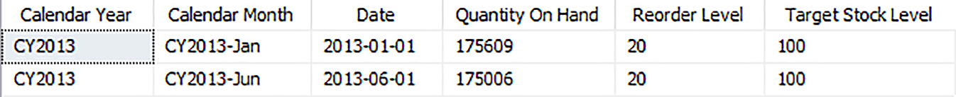
If you remove the Calendar Month and Date attributes from the query, the query returns a single row, as shown in Figure 1-61. The measure values reflect the sum of CY2013-Jan and CY2013-Jun aggregated values for each measure.

This aggregation behavior is incorrect because the measures should reflect the value as of the last inventory date instead of the sum. To change this behavior, perform the following steps:
1. Open the Cube Structure page of the cube designer and set the AggregateFunction property for each of these measures to LastNonEmpty.
2. Deploy the project and then return to the Browser in the cube designer.
3. Click Reconnect in the toolbar, and then add the same three measures to the query window, add Calendar Year from the Date dimension, and set the filter for Stock Item to USB missile launcher (Green) to produce the results shown in Figure 1-62.

Chapter summary
![]() Before you start building a multidimensional database, you should spend time designing a star schema to support business requirements in an OLAP environment. The star schema consists of one or more fact tables and multiple dimension tables that you populate from OLTP systems by using ETL processes. In a multidimensional project that you create in SSDT, you connect to this star schema by creating a data source, and then reference tables in the star schema by creating a data source view. Then you can add dimension objects to your project by using the Dimension Wizard and add a cube by using the Cube Wizard. You can then fine-tune the dimension and cube objects by configuring properties in the dimension and cube designers, respectively. You must deploy your SSDT to create the multidimensional database and its objects on the SSAS server.
Before you start building a multidimensional database, you should spend time designing a star schema to support business requirements in an OLAP environment. The star schema consists of one or more fact tables and multiple dimension tables that you populate from OLTP systems by using ETL processes. In a multidimensional project that you create in SSDT, you connect to this star schema by creating a data source, and then reference tables in the star schema by creating a data source view. Then you can add dimension objects to your project by using the Dimension Wizard and add a cube by using the Cube Wizard. You can then fine-tune the dimension and cube objects by configuring properties in the dimension and cube designers, respectively. You must deploy your SSDT to create the multidimensional database and its objects on the SSAS server.
![]() The storage model you choose determines not only how SSAS stores data, but also what type of data it stores. MOLAP is the default storage model that stores both detail and aggregate data for the optimal data retrieval. SSAS stores only metadata when you use the ROLAP storage model, creates aggregations in the relational data source, and retrieves requests for data from the data source by translating MDX queries into platform-specific SQL statements. ROLAP is beneficial when you need near real-time access to data. SSAS stores aggregate data for the HOLAP storage model and determines at query time whether to retrieve aggregate data from SSAS or from the relational source after converting the MDX query into a SQL statement. HOLAP is useful when most queries require aggregate data.
The storage model you choose determines not only how SSAS stores data, but also what type of data it stores. MOLAP is the default storage model that stores both detail and aggregate data for the optimal data retrieval. SSAS stores only metadata when you use the ROLAP storage model, creates aggregations in the relational data source, and retrieves requests for data from the data source by translating MDX queries into platform-specific SQL statements. ROLAP is beneficial when you need near real-time access to data. SSAS stores aggregate data for the HOLAP storage model and determines at query time whether to retrieve aggregate data from SSAS or from the relational source after converting the MDX query into a SQL statement. HOLAP is useful when most queries require aggregate data.
![]() SSAS supports many different types of dimensional models. The exam tests your knowledge regarding the selection and configuration of the following types:
SSAS supports many different types of dimensional models. The exam tests your knowledge regarding the selection and configuration of the following types:
![]() Fact Use this dimensional model when you want to include a degenerate dimension in your database. On the Dimension Usage page of the cube designer, you must relate the dimension a measure group by using the Fact relationship type.
Fact Use this dimensional model when you want to include a degenerate dimension in your database. On the Dimension Usage page of the cube designer, you must relate the dimension a measure group by using the Fact relationship type.
![]() Parent-child Use this dimensional model when a dimension table includes a foreign-key relationship to itself. Add the column containing the foreign key as an attribute in the dimension and set its Usage property to Parent. Optionally, you can configure properties applicable only to a parent attribute.
Parent-child Use this dimensional model when a dimension table includes a foreign-key relationship to itself. Add the column containing the foreign key as an attribute in the dimension and set its Usage property to Parent. Optionally, you can configure properties applicable only to a parent attribute.
![]() Roleplaying Use this dimensional model when you have a dimension represented multiple times in a fact table in different contexts. For example, you might have Invoice Date and Delivery Date based on the same Date dimension. You create one dimension object in your project, but add the dimension as many times as applicable to the cube. On the Dimension Usage page of the cube designer, you relate each cube dimension to the same measure group by using the Regular relationship type, but define different granularity attributes, which relate to different measure group columns.
Roleplaying Use this dimensional model when you have a dimension represented multiple times in a fact table in different contexts. For example, you might have Invoice Date and Delivery Date based on the same Date dimension. You create one dimension object in your project, but add the dimension as many times as applicable to the cube. On the Dimension Usage page of the cube designer, you relate each cube dimension to the same measure group by using the Regular relationship type, but define different granularity attributes, which relate to different measure group columns.
![]() Reference Use this dimensional model when you need to support slice and dice by a dimension for which no foreign key exists in the fact table although it is related to an intermediate dimension having a foreign key in the fact table. The key attribute for the reference dimension must exist as a non-key attribute in the intermediate dimension. On the Dimension Usage page of the cube designer, you define a Referenced relationship between the reference dimension and the measure group, and specify the intermediate dimension.
Reference Use this dimensional model when you need to support slice and dice by a dimension for which no foreign key exists in the fact table although it is related to an intermediate dimension having a foreign key in the fact table. The key attribute for the reference dimension must exist as a non-key attribute in the intermediate dimension. On the Dimension Usage page of the cube designer, you define a Referenced relationship between the reference dimension and the measure group, and specify the intermediate dimension.
![]() Data mining Use this dimensional model when you want to use a data mining algorithm to create a dimension useful for slicing and dicing, such as clusters of customers. You must first create a data mining model to define the data mining technique and columns to which the data mining algorithm is applied. The Data Mining Wizard allows you to create a dimension in which to store the results and optionally a cube.
Data mining Use this dimensional model when you want to use a data mining algorithm to create a dimension useful for slicing and dicing, such as clusters of customers. You must first create a data mining model to define the data mining technique and columns to which the data mining algorithm is applied. The Data Mining Wizard allows you to create a dimension in which to store the results and optionally a cube.
![]() Many-to-many Use this dimensional model when you need to rollup measures by different dimension attributes without overcounting the results in aggregations. Typically, you must add a bridge table as a measure group to the cube to support this structure and hide the measure group from the cube. On the Dimension Usage page of the cube designer, define a Regular relationship between the dimension and the bridge table and a Many-To-Many relationship between the dimension and the original measure group. You specify the bridge table as the Intermediate Measure group for the many-to-many relationship.
Many-to-many Use this dimensional model when you need to rollup measures by different dimension attributes without overcounting the results in aggregations. Typically, you must add a bridge table as a measure group to the cube to support this structure and hide the measure group from the cube. On the Dimension Usage page of the cube designer, define a Regular relationship between the dimension and the bridge table and a Many-To-Many relationship between the dimension and the original measure group. You specify the bridge table as the Intermediate Measure group for the many-to-many relationship.
![]() Slowly changing dimension Use this dimensional model when you need to track changes to an attribute over time for a Type 2 SCD design. In the dimension design, you must include the key attribute as well as the attribute containing the business key in the source table, and then hide the key attribute by setting its AttributeHierarchyVisible property to False.
Slowly changing dimension Use this dimensional model when you need to track changes to an attribute over time for a Type 2 SCD design. In the dimension design, you must include the key attribute as well as the attribute containing the business key in the source table, and then hide the key attribute by setting its AttributeHierarchyVisible property to False.
![]() Use the Type property for dimension and attribute objects when you need SSAS or client applications to invoke a specific behavior when that object is queried. The most common dimension type to implement is Time, although you should also be familiar with the concepts for implementing the Accounts and Currency dimension types.
Use the Type property for dimension and attribute objects when you need SSAS or client applications to invoke a specific behavior when that object is queried. The most common dimension type to implement is Time, although you should also be familiar with the concepts for implementing the Accounts and Currency dimension types.
![]() After you add a user-defined hierarchy to a dimension, you should review and correct attribute relationships as necessary. A user-defined hierarchy provides a pre-defined navigation path that simplifies cube exploration in a client application. SSAS uses corresponding attribute relationships to optimize both data storage and data retrieval for natural hierarchies.
After you add a user-defined hierarchy to a dimension, you should review and correct attribute relationships as necessary. A user-defined hierarchy provides a pre-defined navigation path that simplifies cube exploration in a client application. SSAS uses corresponding attribute relationships to optimize both data storage and data retrieval for natural hierarchies.
![]() Use the cube designer to add and configure measures and measure groups after initially creating a cube by using the Cube Wizard. Importantly, configure the AggregateFunction and FormatString properties correctly for each measure to ensure values are aggregated appropriately and display legibly in client applications. You can also add calculated measures to include business logic for non-scalar values that are important to business analysis.
Use the cube designer to add and configure measures and measure groups after initially creating a cube by using the Cube Wizard. Importantly, configure the AggregateFunction and FormatString properties correctly for each measure to ensure values are aggregated appropriately and display legibly in client applications. You can also add calculated measures to include business logic for non-scalar values that are important to business analysis.
![]() SSAS includes the following aggregate functions to support semiadditivity: Min, Max, ByAccount, AverageOfChildren, FirstChild, LastChild, FirstNonEmpty, and LastNonEmpty. A semiadditive aggregation adds values together across one dimension, but not across others. Common use cases for semiadditive behavior are financial account reporting and inventory analysis.
SSAS includes the following aggregate functions to support semiadditivity: Min, Max, ByAccount, AverageOfChildren, FirstChild, LastChild, FirstNonEmpty, and LastNonEmpty. A semiadditive aggregation adds values together across one dimension, but not across others. Common use cases for semiadditive behavior are financial account reporting and inventory analysis.
Thought experiment
In this thought experiment, demonstrate your skills and knowledge of the topics covered in this chapter. You can find the answers to this thought experiment in the next section.
Humongous Insurance is a company that sells insurance policies to individual consumers and companies in a single country and has offices in four different regions in this country. The amount for which each insurance policy is sold is called a premium. Each year, the sales manager projects monthly quotas for insurance premiums by region. You have been hired as a BI developer at Humongous Insurance to create an SSAS multidimensional database that enables users to analyze sales and quotas.
The current database environment includes one OLTP system called Sales, and another OLTP system called Quotas. Both databases currently run on SQL Server 2016.
Before you can create the multidimensional database, you must design and populate a data warehouse that can answer the following types of questions:
![]() How many policies have been sold by line of insurance (Personal or Commercial), customer, sales territory, and date?
How many policies have been sold by line of insurance (Personal or Commercial), customer, sales territory, and date?
![]() What is the revenue, cost, profit, and profit percent of policies sold by line of insurance, customer, sales territory, and date?
What is the revenue, cost, profit, and profit percent of policies sold by line of insurance, customer, sales territory, and date?
![]() What is the quota for insurance policies by sales territory and month?
What is the quota for insurance policies by sales territory and month?
To satisfy the business requirements, the multidimensional database must have the following characteristics:
![]() A customer can have multiple policies, but each policy is limited to one customer.
A customer can have multiple policies, but each policy is limited to one customer.
![]() The customer dimension must include the customer name and the customer’s phone number. The phone number must be available for reporting, but not for slicing and dicing operations.
The customer dimension must include the customer name and the customer’s phone number. The phone number must be available for reporting, but not for slicing and dicing operations.
![]() The sales territory dimension must support drilling from region to state/province to city.
The sales territory dimension must support drilling from region to state/province to city.
![]() The date dimension must support drilling from year to month to date.
The date dimension must support drilling from year to month to date.
Based on this background information and business requirements, answer the following questions:
1. Sketch the fact tables, dimension tables, and relationships in the star schema that meets the business requirements.
2. Describe the steps necessary to support the drilldown functionality in the sales territory dimension with optimal query performance.
3. What property do you set to hide the phone number attribute in the customer dimension from slicing and dicing operations, but allows it to be included in the dimension as a member property?
A. AttributeHierarchyOrdered
B. AttributeHierarchyVisible
C. AttributeHierarchyEnabled
D. IsAggregatable
4. What property do you set for each measure to improve the legibility of values in a client application?
A. DataType
B. MeasureExpression
C. AggregateFunction
D. FormatString
5. When you browse the date dimension, you notice the members of the Month attribute sort in alphabetical order. How do you correct this problem?
6. What is the granularity attribute to configure when defining the relationship between the quota measure group and the date dimension?
7. How do you support the profit percentage in your solution design?
A. Add a fact table column and set the FormatString for the new measure to Percent.
B. Create a calculated measure to divide profit by revenue.
C. Add a new measure group to the cube to isolate the measure.
D. Define the MeasureExpression property on a new measure to divide profit by revenue.
8. When you process and then query the cube to view quota by customer, you see the same quota value repeating on each row. What step can you take to prevent the display of these values?
Thought experiment answers
This section contains the solution to the thought experiment.
1. The design for the star schema includes two fact tables—Policy Sales and Policy Quotas—and four dimension tables: Date, Customer, InsuranceLine, and SalesTerritory. The table columns and relationships between the fact tables and dimension tables are shown in Figure 1-63.

2. On the Dimension Structure page of the dimension designer for the sales territory dimension, drag the Year to the Hierarchies pane to create a new user-defined hierarchy, drag the Month attribute to the new hierarchy and drop it below Year, and then drag the Date attribute to the hierarchy and drop it below Month. Right-click the Hierarchy name and type a new name, such as Calendar. On the Attribute Relationships page of the dimension designer, drag the Month attribute and drop it on the Year attribute to arrange the attributes from left to right in the following sequence: Date, Month, and Year. You can set the RelationshipType property for each attribute relationship to Rigid because members do not change in this dimension.
3. The answer is C. AttributeHierarchyEnabled. This attribute property prevents SSAS from storing data for this attribute’s members and hides it from client applications for use in queries on rows, or columns, or as a filter.
Answer A, AttributeHierarchyOrdered, is incorrect because this property only specifies whether the attribute members are ordered. Answer B, AttributeHierarchyVisible, is incorrect because, although it hides the attribute from the client application for slicing and dicing, it does not enable the attribute as a member property. Answer D, IsAggregatable, is incorrect because this property removes the All member from the attribute hierarchy.
4. The answer is D. The FormatString property adds a thousands separator, sets the number of decimal places, or adds symbols such as a currency symbol or percent sign, which makes the values easier to read in client applications.
Answer A, DataType, is incorrect because the data type does not improve the legibility of measure values. Answer B, MeasureExpression, is incorrect because it affects the calculation of a measure, but does not change its appearance. Answer C, AggregateFunction, is also incorrect because it changes how SSAS returns a value for parent members, by summing or counting for example, but does not change the appearance of the measure.
5. For the Month attribute, bind the KeyColumn property to both the Year and Month columns in the source. Also, ensure the OrderBy property is set to Key.
6. Set Month as the granularity attribute. You then map this attribute to the Year and Month columns in the measure group in the Define Relationship dialog box.
7. The answer is B. Add profit as a calculated measure by defining an MDX expression like this:
[Measures].[Profit] / [Measures].[Revenue]
8. Answer A is incorrect because profit percentage is nonadditive and must be calculated at query time, and therefore it cannot be stored in the fact table. Answer C is incorrect for a similar reason. A measure group requires a measure based on a fact table column, and profit percentage cannot be stored in the fact table. Answer D is incorrect because the MeasureExpression calculation is performed at the detail level and then aggregated, which produces an incorrect result. The profit percentage calculation must be based on the aggregated value for profit and divide that value by the aggregated value for revenue.
9. Set the IgnoreUnrelatedDimension on the measure group containing the quota measure to False.