
Niches in NK-Landscapes
Keith E. Mathias [email protected]; Larry J. Eshelman [email protected]; J. David Schaffer [email protected] Philips Research 345 Scarborough Road Briarcliff Manor, NY 10510 (914) 945-6430/6491/6168
Abstract
Introduced by Kauffman in 1989, NK-landscapes have been the focus of numerous theoretical and empirical studies in the field of evolutionary computation. Despite all that has been learned from these studies, there are still many open questions concerning NK-landscapes. Most of these studies have been performed using very small problems and have neglected to benchmark the performances of genetic algorithms (GA) with those of hill-climbers, leaving us to wonder if a GA would be the best tool for solving any size NK-landscape problem. Heckendorn, Rana, and Whitley [7] performed initial investigations addressing these questions for NK-landscapes where N = 100, concluding that an enhanced random bit-climber was best for solving NK-landscapes. Replicating and extending their work, we conclude that a niche exists for GAs like CHC in the NK-landscape functions and describe the bounds of this niche. We also offer some explanations for these bounds and speculate about how the bounds might change as the NK-landscape functions become larger.
1 INTRODUCTION
Introduced by Kauffman in 1989 NK-landscapes [10] are functions that allow the degree of epistasis to be tuned and are defined in terms of N, the length of the bit string and K, the number of bits that contribute to the evaluation of each of the N loci in the string (i.e., the degree of epistasis). The objective function for NK-landscapes is computed as the sum of the evaluation values from N subproblems, normalized (i.e., divided) by N. The subproblem at each locus, i, is given by a value in a lookup table that corresponds to the substring formed by the bit values present at the locus, i, and its K interactors. The lookup table for each locus contains 2K + 1 elements randomly selected in the range [0.0…1.0]. Thus, the lookup table for the entire problem is an N by 2K + 1 matrix.1 When K = 0 the landscape is unimodal and the optimum can easily be found by a simple hill-climber such as RBC (random bit climber) in N + 1 evaluations. When K = N — 1 (the maximum possible value for K), the landscape is random and completely uncorrelated (i.e., knowing the value at any point provides no information about other points in the space, even those that differ from the known point by only a single bit).
NK-landscapes have been the focus of numerous theoretical and empirical studies in the field of evolutionary computation [11,9,8,7,12]. Yet, in spite of numerous studies and all that has been learned about NK-landscapes, there are still many open questions with regard to the ruggedness that is induced on the landscape as K is increased. Particularly, is there enough regularity (i.e., structure) in the landscape for a genetic algorithm (GA) to exploit? Since a hill-climber is the preferred search algorithm at K = 0 and nothing will be better than random search at K = N − 1, the question remains: is there any niche for GAs in NK-landscapes at any value of K?
Heckendorn, Rana, and Whitley’s [7] study, comparing GAs with random bit-climbers, suggested answers to some of these questions for NK-landscapes where N = 100. Figure 1 is replicated here using data supplied by Heckendorn, et al., and shows the performance for three search algorithms on randomly generated NK-landscape problems where N = 100. Figure 1 differs from the figure presented by Heckendorn, et al., in that we present error bars that are ± 2 standard errors of the mean (SEM), roughly the 95% confidence interval for the mean. Figure 1 also provides an inset to magnify the performance values in the interval 3 ≤ K ≤ 12. Heckendorn, et al. observed:
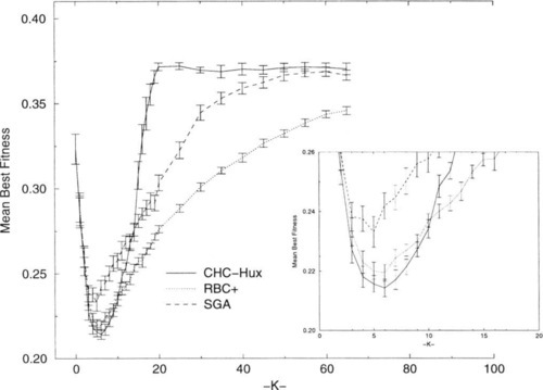
• The enhanced hill-climber, RBC + [7], performed the best of the algorithms they tested.
• A niche for more robust GAs, like CHC [3], mav not exist at all since CHC generally performed worse than a robust hill-climber and the performance of CHC becomes very poor when K ≥ 12.
• The performance of the simple genetic algorithm (SGA) is never competitive with that of other algorithms.
Their work raises several questions: Why are the average best values found by the algorithms decreasing when 0 ≤ K ≤ 5, and why are the average best values found by the algorithms increasing for K > 6? Can w’e determine if and when any of these algorithms are capable of locating the global optima in NK-landscapes? What does the dramatic worsening in the average best values found by CHC, relative to the hill-climbers, for K > 10 tell us about the structure of the NK-landscape functions as K increases. What is the significance of CHC’s remarkably stable performance for K > 20? And perhaps most interesting, is there a niche where a GA is demonstrably better than other algorithms in NK-landscapes?
2 THE ALGORITHMS
In this work we have begun to characterize the performance niches for random search, CHC using the HUX [3] and two-point reduced surrogate recombination (2X) [1] operators, a random bit-climber, RBC [2], and an enhanced random bit-climber, RBC + [7]. The random search algorithm we tested here kept the string with the best fitness observed (i.e., minimum value) from T randomly generated strings, where T represents the total allotted trials. The strings were generated randomly with replacement (i.e., a memoryless algorithm).
CHC is a generational style GA which prevents parents from mating if their genetic material is too similar (i.e., incest prevention). Controlling the production of offspring in this way maintains diversity and slows population convergence. Selection is elitist: only the best M individuals, where M is the population size, survive from the pool of both the offspring and parents. CHC also uses a “soft restart” mechanism. When convergence has been detected, or the search stops making progress, the best individual found so far in the search is preserved. The rest of the population is reinitialized: using the best string as a template, some percentage of the template’s bits are flipped (i.e., the divergence rate) to form the remaining members of the population. This introduces new genetic diversity into the population in order to continue search but without losing the progress that has already been made. CHC uses no other form of mutation.
The CHC algorithm is typically implemented using the HUX recombination operator for binary representations, but any recombination operator may be used with the algorithm. HUX recombination produces two offspring which are maximally distant from their two parent strings by exchanging exactly half of the bits that differ in the two parents. While using HUX results in the most robust performance across a wide variety of problems, other operators such as 2X [1] and uniform crossover [13] have been used with varying degrees of success [5,4]. Here, we use HUX and 2X and a population size of 50.
RBC, a random bit climber defined by Davis [2], begins search with a random string. Bits are complemented (i.e., flipped) one at a time and the string is re-evaluated. All changes that result in equally good or improved solutions are kept. The order that bit flips are tested is random, and a new random testing order is established for each cycle. A cycle is defined as N complements, where N is the length of the string, and each position is tested exactly once during the cycle. A local optimum is found if no improvements are found in a complete test cycle. After a local optimum has been discovered, testing may continue until some number of total trials are expended by choosing a new random start string.
RBC + [7] is a variant of RBC that performs a “soft restart” when a local optimum is reached. In RBC +, the testing of bit flips is carried out exactly as described for RBC. However, when a local optimum is reached, a random bit is complemented and the change is accepted regardless of the resulting fitness. A new testing order is determined and testing continues as described for RBC. These soft restarts are repeated until 5*N changes are accepted (including the bit changes that constituted the soft restarts), at which point a new random bit string is generated (i.e., a “hard restart”). This process continues until the total trials have been expended.
3 THE NK OPTIMA
One striking characteristic of the performance curves in Figure 1 is the dramatic decrease in the average best objective values found by all of the search algorithms when 0 ≤ K ≤ 6 and the increase in the average best values found by all of the search algorithms when K > 6. One may reasonably ask whether these trends represent improvement in the performance of the algorithms followed by worsening performances or whether they indicate something about the NK-landscapes involved.
A hint at the answer may be seen by looking ahead to Figure 4 where a plot of the performance of a random search algorithm shows the same behavior (i.e., decreasing objective values) when K ≤ 6 but levels off for higher K. The basic reason for this can be explained in terms of expected variance in increasing sample sizes. The fitness for an NK-landscape where N = 100 and K = 0 is simply the average of 100 values, where the search algorithm chooses the better of the two values available at each locus. When K = 1 the fitness is determined by taking one of four randomly assigned values; the four values come from the combinations of possible bit values for the locus in question and its single interactor (i.e., 00, 01, 10, and 11). In general, averages of more random numbers will have more variance, leading to more extreme values. However, this ignores the constraints imposed by making a choice at a particular locus and how that affects the choices at other loci. We expect that this would at least cause the downward slope of the curve to level off at some point, if not rise, as K increases. This is consistent with the findings of Smith and Smith [12] who found a slight but significant correlation between K and the minimum fitness.
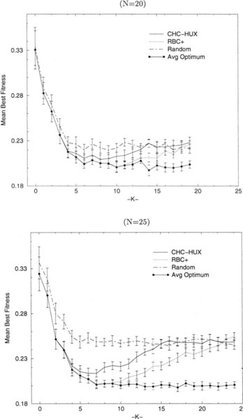
We performed exhaustive search on 30 random problems, at every K, for 10 ≤ N ≤ 25. Figure 2 shows the average global optima (Avg Optimum) and the performance (average best found) for CHC-HUX, RBC +, and random search allowing 200,000 trials for N = 20 and N = 25. We see that the average of the global optima decreases as K increases from 0 to 6 and then it remains essentially constant for both N = 20 and N = 25.2 We conjecture that this pattern also holds for larger values of N. Also in Figure 2, we see the answer to our second question concerning the values of the optimal solutions in an NK-landscape where K > 6. The increasing best values found by the algorithms when K > 6 indicates that search performance is in fact worsening, and not that the values of the optima in the NK-landscapes are increasing.
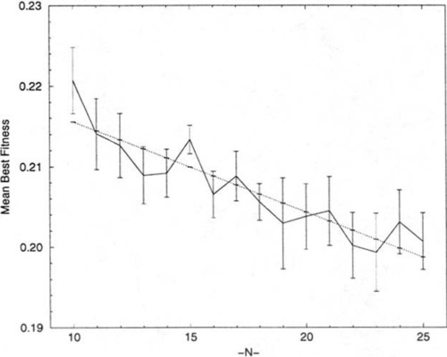
If we accept that the optima for these NK-landscapes have essentially reached a minimum when K > 6, then we can examine how this minimum vanes with N by examining only the optima at K = N − 1. Figure 3 presents the average global optima for 30 random problems at K = N − 1 for the range 10 ≤ N ≤ 25. The values of N are shown on the X-axis. And a linear regression line, with a general downward trend3 and a correlation coefficient of 0.91, has been inserted. This observation is consistent with the Smith and Smith [12] finding of a correlation between N and best average fitnesses in NK-landscapes.
4 NK NICHES
Comparing algorithm performances on NK-landscape functions where the optima are known, although useful, limits us to small N problems where exhaustive search is still practical. One of the contributions of Heckendorn, et al. [7] was that they made their comparisons for N = 100, a much larger value of N than used in most other studies. As a starting point for extending the comparisons made by Heckendorn, et al. for larger N problems, we performed independent verification experiments. We tested CHC using the HUX and 2X recombination operators, as well as RBC, RBC + and random search on NK-landscapes where N = 100, generating thirty random problems for each value of K tested.4 We tested all values for K in the range 0 ≤ K ≤ 20, values in increments of 5 for the range 25 ≤ K ≤ 95, and K = 99. The total number of trials allowed for each experiment was 200,000. Figure 4 shows the results of our verification experiments and the behavior of random search. Figure 4 exhibits the same properties as those observed by Heckendorn, et al., and shown in Figure 1.
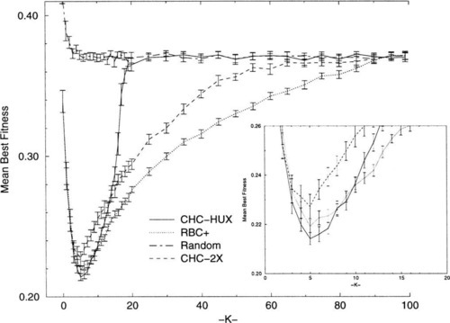
Figure 4 shows that when N = 100, the performance of each of the algorithms becomes indistinguishable from random search at some point. CHC-HUX is the first to do so (at K = 20). Figure 4 also shows that CHC-HUX performs better than RBC + in the region 1 ≤ K ≤ 7 but the performance of CHC-HUX is better than RBC + by more than two standard errors only in the region 4 ≤ K ≤ 7.5 Furthermore, it is interesting to note that the N = 100 problems axe surprisingly difficult even for low values of K. For example, none of the algorithms tested can consistently locate the same best solution in 30 repetitions of the same problem for most of the K = 2 problems generated.
CHC-2X never performs as well as CHC-HUX in the range 3 ≤ K ≤ 13, but the performance of CHC-2X does not degrade as rapidly as CHC-HUX when K ≤ 15, and the performance of CHC-2X does not regress to random search until K ≥ 70. 2X produces offspring that are much more like their parents than HUX. This results in much less vigorous search than when using HUX. Thus, the performance of CHC-2X is more like that of the hill-climbers. Furthermore, by comparing Figure 1 with Figure 4 it can be seen that CHC-2X performs at least as well as the SGA (using one-point crossover) over all K’s and usually much better.
RBC + exhibits the most robust performance over all K’s when N = 100, as observed by Heckendorn, et al., and performs significantly better than CHC-HUX when K ≥ 11. When N = 100, RBC performs better then RBC + for K = 1 and is statistically indistinguishable from RBC + when K ≥ 20.6 The performance of both hill-climbers becomes indistinguishable from random search when K ≥ 90.
Comparing the performances of all of these algorithms on NK-landscapes where N = 100 indicates that no algorithm performs better than all of the others for all values of K (i.e., dominates). Rather, we see niches where the advantage of an algorithm over the others persists for some range of values of K. These observations are consistent with what we saw for low N in the previous section. For example, re-examination of Figure 2 shows that the performance of CHC-HUX becomes indistinguishable from that of random search at lower values of K than does the performance of the hill-climbers, which is consistent with the behavior of CHC-HUX when N = 100 (Figure 4). However, there does not appear to be any niche in which CHC-HUX performs better than RBC + when N = 20 or N = 25, as shown in Figure 2. In fact, CHC-HUX is unable to consistently find the optimum solution even when K is quite small (i.e., K ≥ 3 for N = 20 and K ≥ 1 for N = 25) as indicated by the divergence of the lines for CHC-HUX performance and the average optimum. RBC +, on the other hand, consistently finds the optimum for much larger values of K.
Table 1 shows the highest value of K at which CHC-HUX, CHC-2X, RBC +, and RBC are able to consistently locate the optimal solution for all 30 problems in the range 19 ≤ N ≤ 25. CHC-2X, RBC, and RBC + are all able to consistently locate the optimum at higher values of K than CHC-HUX when 19 ≤ N ≤ 25. And RBC is better at locating the optimum consistently than any of the other algorithms for this region. This is critical in that most work testing GA performance on NK-landscapes has been done using small values for N and often do not include hill-climbers as benchmarks. The performance information in Table 1 makes it clear that there is not a niche for even a robust GA like CHC in NK-landscapes where N is small. This indicates that if niches exist for different algorithms in the NK-landscapes they will have to be characterized in both the N and K dimensions.
Table 1
Highest value of K at which CHC-HUX, CHC-2X, RBC and RBC + consistently locate the optimum solution.
| N | 19 | 20 | 21 | 22 | 23 | 24 | 25 |
| CHC-HUX | 1 | 3 | 1 | 1 | 1 | 1 | 1 |
| CHC-2X | 8 | 5 | 6 | 5 | 3 | 3 | 4 |
| RBC + | 9 | 9 | 7 | 6 | 7 | 6 | 6 |
| RBC | 11 | 9 | 9 | 8 | 9 | 7 | 6 |
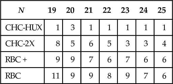
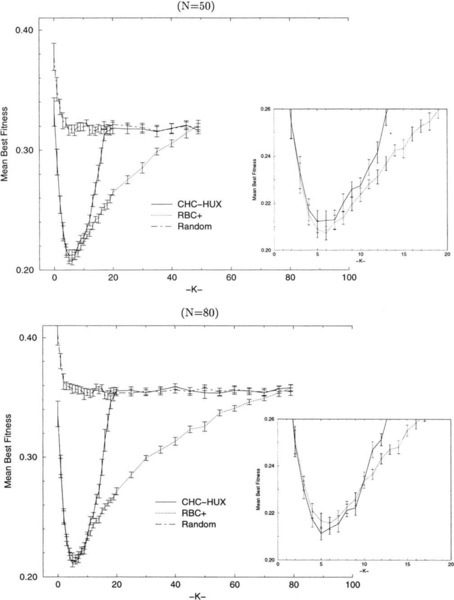
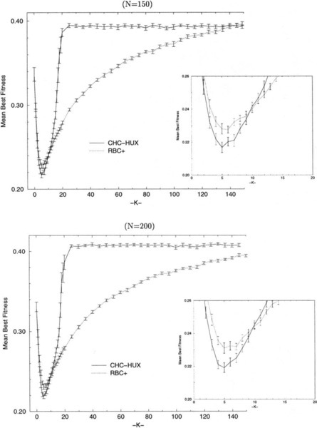
Figure 5 shows the performances for CHC-HUX, RBC +, and random search on NK- landscapes where N = 50 and N = 80, for all values of K where K ≤ 20, in increments of 5 for 25 ≤ K ≤ N − 5, and for K = N − 1. Thirty random problems were generated for each (N, K) combination tested.7 At N = 50, RBC + still performs better than CHC-HUX for all K’s tested. But at N = 80, K = 4 and K = 5 we see the first hint of a niche for CHC-HUX in NK-landscapes (i.e., CHC-HUX performs significantly better than RBC +). Figure 4 showed that the niche where CHC-HUX performs best extended to K = 7 and Figure 6 shows that the niche for CHC-HUX also includes up to K = 9 when N = 150 and K = 10 when N = 200.
Figures 7(a-d) indicate those NK-landscapes where one algorithm performs better than another, based on the average best values found after 200,000 trials for all of the values of N and K that we have tested (i.e., 19 ≤ N ≤ 25 in increments of 1, 30 ≤ N ≤ 100 in increments of 10; K was tested in increments of 1 for 0 ≤ K ≤ 20, and in increments of 5 for 20 ≤ K ≤ N − 5, and K = N − 1). Unfilled circles represent NK-landscapes where one algorithm performs better than another, while filled circles indicate significantly (i.e., > (2 * SEM)) better performance by one algorithm over another. The points that were tested at which no circle is present indicates that the algorithms being compared were able to locate the same local optima (i.e., tied). These points occur occasionally and only when K ≤ 9 and N ≤ 30. Figure 7-a shows those NK-landscapes where RBC + performs better/significantly better than RBC while Figure 7-b shows those NK-landscapes where RBC performs better/significantly better than RBC +. Figure 7-c shows the NK-landscapes where RBC + performs better than CHC-HUX, and Figure 7-d indicates the NK-landscapes where CHC-HUX performs better/significantly better than RBC +.
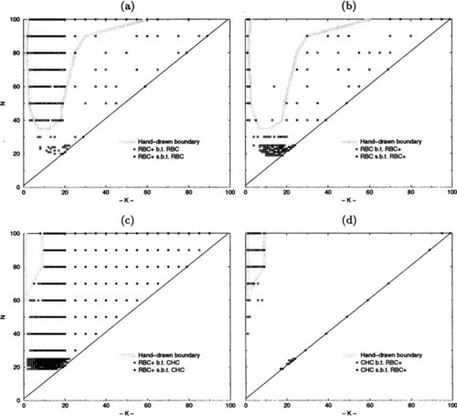
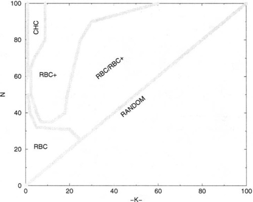
The information presented in Figures 7(a-d) gives a coarse pairwise comparison of the NK-landscapes where various algorithms might be useful. While there are regions where no algorithm seems to be the best, there are certainly regions where one algorithm is a better choice than the others and some regions where one algorithm is much worse than the other two. Figure 8 summarizes those regions where each algorithm is observed to exhibit an advantage over the others. Additional analysis information (i.e., trials to find the best local minima when the local minima found are the same for the algorithms) was sometimes necessary to make this determination, as explained in the next section.
5 DISCUSSION
As Figures 7(c-d) indicate, the GAs niche in the universe of NK-landscapes is quite small. And not all GAs even have a niche: as we have seen, the SGA, as well as CHC-2X, are completely dominated by RBC +. On the other hand, CHC-HUX does dominate RBC + for a small region, but its performance quickly deteriorates to no better than random search for K ≥ 20. What does this tell us about CHC-HUX and about the structure of NK-landscapes?
There are at least two types of landscapes where a hill-climber like RBC should have an advantage over a GA: when the landscape is very simple or when it is very complex. By a simple landscape we mean one that has two properties. First, the landscape is such that the catchment basin of the global optimum (or some other very good point) is large enough that there is a good chance that a randomly chosen point will fall in this basin, and thus it will not take too many random restarts before the hill-climber lands in the right basin. Second, the paths to the bottoms of the catchment basins are not too long. Of course, there can be some tradeoff between these two conditions. The expected cost of finding the global optimum is a product of how many iterations it takes before the hill-climber is likely to fall in the right basin, and how many cycles the average climb will take before no more improvements can be found.
If the hill-climber allows for soft restarts, like RBC +, then an additional condition needs to be added: many of the local optima which are good are very neax (in Hamming distance) to the global optimum.8 This means that if the hill-climber gets stuck in one of these regions, exploring other local optima in this region (via soft restarts) will be useful. Again there will be tradeoffs. If there are not that many local optima relative to the total number of trials the hill-climber is allowed, then the overhead of exploring nearby local optima may penalize a hill-climber with soft restarts (like RBC +).
Of course, the easiest problem for a hill-climber is a bitwise linear problem like the One-max problem. The K = 0 problems fall in this category, and, as expected, RBC and RBC + can solve these problems in one cycle. For other problems, a hill-climber may get trapped in a local minimum, but for low N (e.g., 20) and low K (e.g., K = 1 or K = 2) we would expect that RBC and RBC + will do fairly well. In fact, RBC should have a competitive advantage over a GA in these types of problems because it does not waste evaluations exploring neighboring local optima. However, as N is increased, the number of local optima will increase, so that even for AT = 1, RBC and RBC + will lose their advantage over CHC.
The break even point for K = 1 problems is at about N = 30. At N = 30 RBC, RBC + and CHC-HUX all find the same best solutions for all 30 problems. RBC and CHC take about the same number of trials to find these solutions, whereas RBC + takes about three times as many. At N = 40 and K = 1, RBC and CHC find the same set of solutions, but RBC takes about two and half as many trials, whereas RBC + sometimes fails to find solutions as good as RBC and CHC and takes about three times as many trials as RBC. As N increases this trend continues for K = 1 and K = 2, with CHC dominating RBC, and RBC dominating RBC +. The reason RBC + does relatively poorly in this region is that it is paying a price for the overhead of its soft restarts with very little gain. The local minima are in large attraction basins so that soft restarts tend to repeatedly find the same solutions, thus wasting evaluations. RBC, on the other hand, is able to explore many more local minima than RBC + in the same number of evaluations. Although CHC-HUX suffers from the same problem as RBC + (its soft restarts tend to bring it back to the same solution) this problem does not arise for low K, since CHC-HUX is usually able to find the good solutions for these problems without any restarts. So on these problems two very different strategies work fairly well: quickly exploring many local minima (RBC) or slowly exploring the global structure, gradually focusing in on the good local minima (CHC-HUX). As N increases, the probability of exploring all the local minima decreases, and the second strategy gains an advantage.
A more detailed look at the RBC runs on the N = 30, K = 1 problems (i.e., 30 different problems) shows that in 200,000 trials, constituting about 2200 restarts, RBC finds, on average, about 33 different local optima, although this varies across problems from a low of 8 to a high of 145. However, RBC is better at finding the best solution than this might indicate: RBC finds the best solution, on average, in about 11% of its restarts, although, again, this varies across problems from a low of 1% to a high of 27%.
The second type of landscape that will give a hill-climber a competitive advantage over a G A is a complex landscape. The particular type of complex landscape we have in mind here is one where there are many local optima of varying depths, but a good local optimum does not indicate that neighboring local optima are any good. In other words, there is structure at the fine grain level but not at a more coarse grain level, so finding good solutions at the local level tells one nothing about good solutions at the regional level. Such a problem will be very difficult for a GA since crossing over two good, but unrelated solutions, will very likely produce poor solutions. This tendency will be exacerbated by HUX and incest prevention. When presented with a surface characterized by rampant multi-modality with little or no regional structure, CHC-HUX is reduced to random search. A hill-climber, on the other hand, will do much better because of its ability to search many more attraction basins. Of course, it will not be able to find the global optimum, unless it is a very small search space, but it will, simply by brute force, search many more basins, and thus do better. Furthermore, the ability of RBC + to search neighboring basins will give it an advantage over RBC for larger N. Since RBC will only be able to search a small fraction of all the local minima, the ability to search deeper in each region explored will give RBC + an advantage. However, as K increases and the regional structure disappears, RBC + starts to lose its advantage over RBC and the performance of the two algorithms become indistinguishable.
Finally, for very high K, e.g., K = N − 1, CHC-HUX has an advantage again. This can be seen in Figures 7(d) where CHC-HUX has many “wins” along the diagonal. The reason for this is that for these NK-landscapes, CHC-HUX is better at random search than the hill- climbers. Both RBC and RBC + must waste evaluations each cycle ascertaining that there are no more improvements possible by a single bit-flip. CHC-HUX, on the other hand, will rarely generate solutions for such high K that are identical to previously generated solutions.
In summary, perhaps the reason that CHC-HUX’s niche in the universe of NK-landscapes is small is because the region of “effective complexity” is small. Information theory would call bit strings of all zeros/ones the most simple, and completely random strings the most complex. Gell-Mann [6] has proposed the notion of “effective complexity” that would reach its maximum somewhere between these extremes and would more accurately reflect our intuitions about complexity. Figures 9-11 illustrate in various ways how this critical region affects the algorithms differently. Figure 9 shows the number of cycles in RBC per restart over K for a set of representative N’s. Note that all the N curves peak between K of 3 and 6, with 6 being the peak value for N = 100. The minimum number of cycles is two, a second pass being required to verify that there are no more changes that lead to an improvement. As expected, all N with K = 0 require only two cycles. Furthermore, the number of cycles per restart for all N approaches two as K approaches N − 1. As the number of local optima increase, the average attraction basin gets smaller and shallower. The intriguing point is that the measure of cycles per restart peak in the same region where CHC-HUX has a competitive advantage, possibly indicating effective complexity.
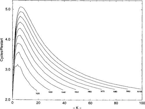
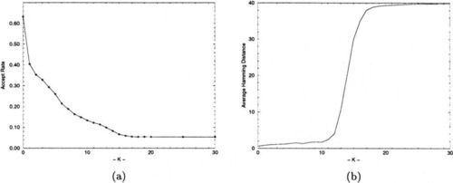
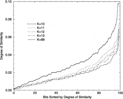
Figure 10-a shows the acceptance rates for CHC-HUX on N = 100 NK-landscapes for various K. The acceptance rate is the fraction of offspring generated that are fit enough to replace some worse individual in the population. As a rule of thumb, CHC-HUX does best on problems where its acceptance rate is around 0.2. If the acceptance rate is very high, the problem may be better suited for a hill-climber like RBC. For example, on the One-max problem the acceptance rate is around 0.6. On the other hand, if the acceptance rate is below 0.1, then this usually indicates that the problem will be difficult for CHC. Sometimes this can be remedied by either using a less disruptive crossover operator or a different representation. As can be seen in Figure 10-a, the acceptance rates deteriorate to about 0.055 by K = 18. An acceptance rate this low indicates that the members of the population have very little common information that CHC-HUX can exploit, and that crossover is, in effect, reduced to random search. In fact, most of the accepts come in the first few generations after either a soft restart or creation of the initial population, where a population of mostly randomly generated solutions is being replaced. Interestingly, the acceptance rates fall much more slowly when CHC uses 2X instead of HUX as its crossover operator. As we noted earlier 2X does much better than HUX in the range where K ≥ 15, although not as well as HUX in the range where 3 ≤ K ≤ 13.
An even more dramatic illustration of this phenomenon can be seen in Figure 10-b, which shows the degree to which CHC-HUX’s population is converged immediately before it restarts. CHC has two criteria for doing a soft restart: (1) All the members of the population have the same fitness value. (2) The incest threshold has dropped below zero.9 If CHC is having difficulty generating new offspring that axe fit enough to be accepted into the population, then the incest threshold will drop to zero before the population has converged. Figure 10-b shows the average Hamming distance over K between randomly paired individuals in the population at the point of a restart, averaged over all restarts for all experiments for the N = 100 problems where 0 ≤ K ≤ 30. After K ≥ 12 the amount of convergence rapidly deteriorates, leveling off at about 40. Note that this is only slightly less than 50, the expected Hamming distance between two random strings of length 100.
Figure 11 shows the degree of similarity of the local optima found by RBC over K for the N = 100 problems. For each K the solutions for 2000 hill-climbs are pooled and the degree of similarity is determined for each locus. These loci are sorted according to the degree of similarity, with the most similar loci on the right. Note that by about K = 13, the results are indistinguishable from the amount of similarity expected in random strings, represented here by K = 99. This, as we have seen, is the point where CHC-HUX rapidly deteriorates, although CHC does somewhat better than random search until K ≥ 20. In effect, this is showing that there is very little in the way of schemata for CHC to exploit after K = 12, the point where it is over taken by RBC +.
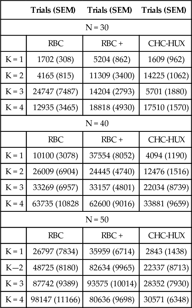
Finally, Table 2 shows the mean number of trials to the best solution found and the standard error of the mean for CHC-HUX, RBC, and RBC + in the region where their three niches meet. Note that CHC usually requires fewer trials before it stops making progress. While we have not yet performed the tests needed to support conclusions for other values, we speculate that if fewer trials were allotted for search than the 200,000 used for the experiments presented in this paper, the niche for CHC-HUX will expand at the expense of the hill-climbers. This results from the hill-climber’s reliance on numerous restarts. Conversely, increasing the number of trials allowed for search should benefit the hill-climbers while providing little benefit for CHC-HUX. CHC-HUX’s biases are so strong that they achieve their good effects (when they do) very quickly. Allowing large numbers of “soft-restarts” for CHC-HUX (beyond the minimum needed for the problem) usually does not help.
Table 2
Average trials to find best local minima discovered (not necessarily the optimum) and the standard error of the mean (SEM).
| Trials (SEM) | Trials (SEM) | Trials (SEM) | |
| N = 30 | |||
| RBC | RBC + | CHC-HUX | |
| K = 1 | 1702 (308) | 5204 (862) | 1609 (962) |
| K = 2 | 4165 (815) | 11309 (3400) | 14225 (1062) |
| K = 3 | 24747 (7487) | 14204 (2793) | 5701 (1880) |
| K = 4 | 12935 (3465) | 18818 (4930) | 17510 (1570) |
| N = 40 | |||
| RBC | RBC + | CHC-HUX | |
| K = 1 | 10100 (3078) | 37554 (8052) | 4094 (1190) |
| K = 2 | 26009 (6904) | 24445 (4740) | 12476 (1516) |
| K = 3 | 33269 (6957) | 33157 (4801) | 22034 (8739) |
| K = 4 | 63735 (10828 | 62600 (9016) | 33881 (9659) |
| N = 50 | |||
| RBC | RBC + | CHC-HUX | |
| K = 1 | 26797 (7834) | 35959 (6714) | 2843 (1438) |
| K—2 | 48725 (8180) | 82634 (9965) | 22337 (8713) |
| K = 3 | 87742 (9389) | 93575 (10014) | 28352 (7930) |
| K = 4 | 98147 (11166) | 80636 (9698) | 30571 (6348) |
6 CONCLUSIONS
We have presented results of extensive empirical examinations of the behaviors of hill- climbers and GAs on NK-landscapes over the range 19 ≤ N ≤ 100. These provide the evidence for the following:
• While the quality of local minima found by both GAs and hill-climbers deteriorates as both N and K increase, there is evidence that the values of the global optima decrease as N increases.
• There is a niche in the landscape of NK-landscapes where a powerful GA gives the best performance of the algorithms tested; it is in the region of N > 30 for K = 1 and N > 60 for 1 ≤ K < 12.
• NK-landscapes are uncorrelated when K = N − 1, but our evidence shows that the structure in NK-landscapes deteriorates rapidly as K increases, becoming such that none of the studied algorithms can effectively exploit it when K > 12 for N up to 200. This K-region is remarkably similar for a wide range of N’s.
• Finally, the advantage that random bit-climbers enjoy over CHC-HUX depends on three things: the number of random restarts executed (a function of the total number of trials allotted and the depth of attraction basins in the landscape), the number of attraction basins in the space, and the size of the attraction basin containing the global optimum relative to the other basins in the space. If the total trials allowed is held constant, then as N increases CHC-HUX becomes dominant for higher and higher K.
Acknowledgments
We would like to thank Robert Heckendorn and Soraya Rana for their help and cooperation throughout our investigation. They willingly provided data, clarifications and even ran validation tests in support of this work.