Chapter 6: Forecasting by Exponential Smoothing of Seasonal Series

6.1 Seasonal Exponential Smoothing

6.2 Using the Winters Method for Seasonal Forecasting

6.3 Forecasting the Number of Overnight Stays by US Citizens at Danish Hotels

6.4 Forecasting Using Additive Seasonal Exponential Smoothing with PROC ESM

6.5 Forecasting US Retail E-Commerce Using the Winters Method

6.6 Forecasting the Relative Importance of E-Commerce by PROC ESM

6.7 Forecasting the Relative Importance of E-Commerce Using a Transformation in PROC ESM

6.1 Seasonal Exponential Smoothing

Seasonal factors can be included in forecasts derived from the exponential smoothing method by extending the basic idea behind exponential smoothing in order to allow for seasonal behavior. In this and the following section, these methods are outlined in theory. The sections that follow them are devoted to various examples. These examples cover many practical applications, which demonstrate the facilities offered by SAS procedures such as PROC ESM.

Seasonality is included in exponential smoothing by introducing a new multiplicative seasonal factor so that the hypothetical true level is . The seasonal factor for monthly data is dependent on the month, and the index t could reflect a constant value each year for the month of May . The factor is considered as the level of the time series apart from any seasonality. The seasonal factors vary around 1 and explain nothing more about the actual level but the monthly structure. In order to extend the model, these seasonal factors are made more flexible by letting them change over time by a mechanism of the same form as exponential smoothing. For that reason, an additional index has to be introduced so that denotes the seasonal factor for the month of May, calculated by knowledge of the time series up to the time index u.

Using this notation, the prediction beyond the latest observation becomes

where time index T+i corresponds to the month of May.

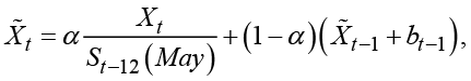
The value of the level , assuming that t corresponds to the month of May, is calculated by a formula similar to that of exponential smoothing

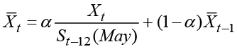
where is the seasonal component for the month of May, which is calculated using only observations up to time t - 12. The formula is a simple exponential smoothing of the seasonally adjusted series .

Still, for the time index t being the month of May, the seasonal component for the present observation is updated to as a weighted average of a previously defined value and previously calculated values of estimated seasonal factors, , for the months of May in previous years

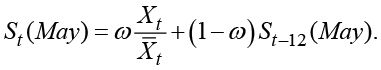
This is again an application of the basic idea of exponential smoothing, this time applied to the series of estimated seasonal factors for the months of May. For the weighted average, a new weight ω is applied as the changes to the seasonality could differ from the changes in level and trend. Values of ω close to 0 correspond to a slowly varying seasonal pattern. Values of ω close to 1 correspond to a very unstable seasonal structure.

The initial values for the seasonal components are usually derived as the ratio of the first two months of May in the series divided by the overall average of the first 24 observations. Forecasting in a series with seasonality is most reliable when many seasonal periods are present in the observation period.

If a trend is included, the true level is easily replaced by the calculated true level obtained by double exponential smoothing of the series of seasonal adjusted observations . Triple smoothing could also be applied in the same way.

In PROC ESM, the seasonal smoothing parameter is estimated along with the other smoothing parameters by minimizing the sum of squares of forecast errors in the observation period, as described in Section 5.10.

Another possibility is to elaborate the same idea by using an additive seasonal structure defined by . If this additive version is applied, an exact moving average representation exists and confidence limits are then easily calculated, as explained in Section 5.7. In the multiplicative formulation, no such representation exists and the confidence limits are calculated using approximating representations.

6.2 Using the Winters Method for Seasonal Forecasting

The Holt formulation of linear exponential smoothing could be combined with the idea of seasonal exponential smoothing. This is easily done by using the updating formulas in the linear smoothing algorithm not for the original series , but instead for the seasonal adjusted series , where is a seasonal factor. See Section 6.1. Considering monthly data and thinking about the month of May as in Section 6.1, the updated equation becomes

and

This multiplicative version could again easily be revised into an additive version by substituting for as an expression for the seasonal adjusted observation at time index t. The multiplicative version is preferable for most series with a clear trend component because the seasonal variation is relative to the level and not just an additive component. See the example in Section 6.5. For series without any important trends, estimating a trend component using the Winters method introduces a risk of misleading predictions along an insignificant trend that is fitted by coincidence. In this case, an additive seasonal forecasting procedure is preferable, as seen in Section 6.4.

All such procedures are named after Winters, or Holt and Winters; see Harvey (1984). Often the point that the forecasting method includes three parameters is stressed, and the method is named the “Winters three-parameter method.”

6.3 Forecasting the Number of Overnight Stays by US Citizens at Danish Hotels

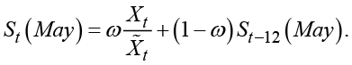
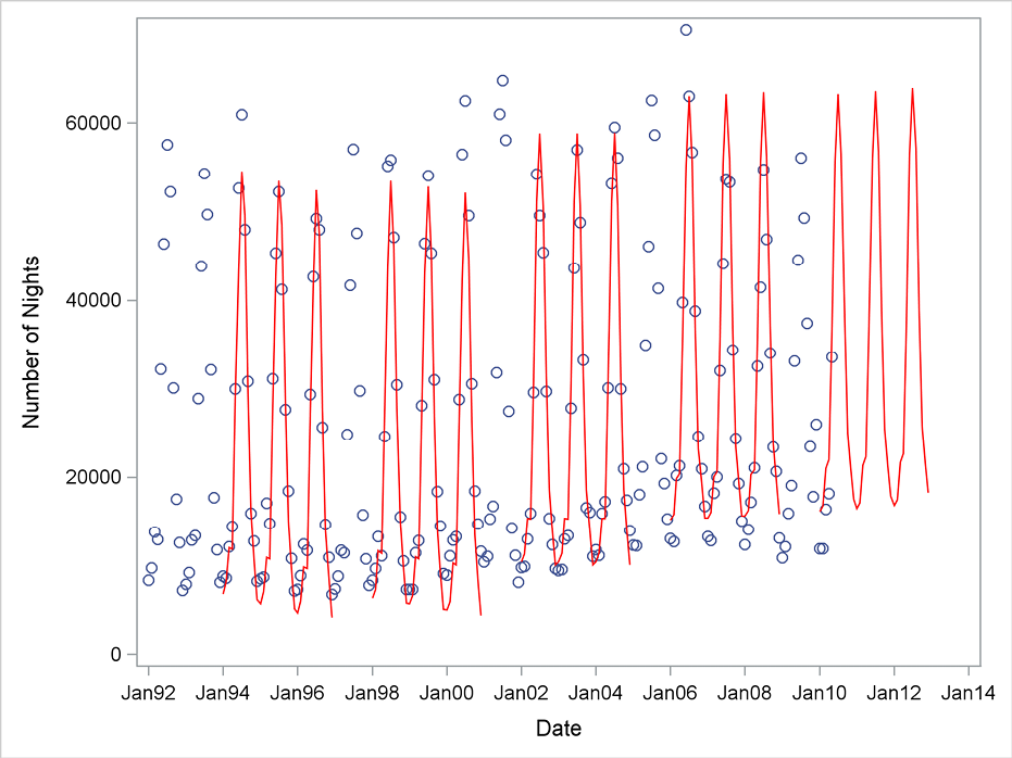
In this section, the monthly number of nights that US citizens stayed in Denmark is used as an example of automatic forecasting of a time series with a seasonal structure. The data series is provided by the official Danish Statistical Office, based on reports by the hotels. When the series of overnight stays at hotels is observed as a monthly time series, a clear seasonal pattern emerges. A large number of tourists in the summer months is seen, and a smaller number of overnight stays in the winter months is dominated by business trips.

The series is observed from January 1992 to May 2010, giving a total of 221 observations. Some outliers are present in the series, possibly because of major conferences and political occasions. The series is plotted in Figure 6.1 using the SGPLOT procedure. Program 6.1 also provides a more detailed plot, Figure 6.2, of the variation within a year. The level of the time series could for all practical purposes be considered as constant, which does not exclude the possibility of minor systematic trends for a shorter span of years. The seasonal pattern is very explicit and almost constant from year to year, even if some irregularities exist. These irregularities could be regarded as outliers, especially the observation from December 2009 which probably was due to a huge international conference in Copenhagen that even the American president attended.

Program 6.1 Plotting the overnight stay time series

PROC SGPLOT data=sasts.hotel;
series x=date y=number_of_nights/markers;
xaxis values=(‘1jan92’d to ‘1jan11’d by year);
run;
quit;
PROC SGPLOT data=sasts.hotel;
series x=month y=number_of_nights/markers group=year;
xaxis values=(1 to 12 by 1);
where year<2010 and year>2006;
run;
quit;

Figure 6.1 Number of overnight stays by US citizens at Danish hotels

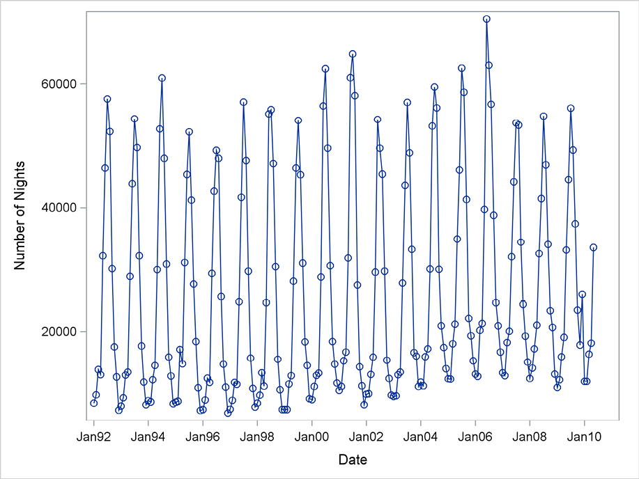
Figure 6.2 The seasonal structure for monthly numbers of overnight stays

In PROC ESM, forecasts of this seasonal time series could be generated by many methods. One simple possibility is the multiplicative seasonal exponential smoothing method, which is exactly as the forecasts are generated when using the simple method described in Section 6.1. This method is obtained by the option method=multseasonal in Program 6.2. The options in the procedure state that the estimated smoothing parameters are written to the output window and that all relevant plots are generated in the ODS Graphics System.

Program 6.2 An application of multiplicative exponential smoothing in PROC ESM

ods graphics;
PROC ESM data=sasts.hotel print=estimates plot=all lead=24;
id date interval=month ;
forecast number_of_nights/method=multseasonal;
run;
ods graphics off;

In this code, the time index of the series is stated in the ID statement, and the seasonality is specified by the option interval=month. The option lead=24 specifies the number of forecasts to be generated. The default is lead=12.

Estimates of the weight parameters from the smoothing algorithm are printed in the procedure output (Output 6.1). This print option must be specified in the procedure call in Program 6.2 because PROC ESM produces no printed output by default. The estimates are α = 0.11 and ω = 0.53. These estimates are rather precise when judged from the reported standard deviations so that even the estimated value α = 0.11 is significantly positive. The weight α = 0.11 is close to 0, which indicates that the series has a rather constant level such that even very old observations contain information about the present level. The seasonal weight parameter ω = 0.53 is substantially different from 0, so the seasonal structure is allowed to vary. However, because the value is also much smaller than 1, the seasonal factors are not extremely fluctuating but only moderately varying.

Output 6.1 Estimates by PROC ESM for the smoothing parameters

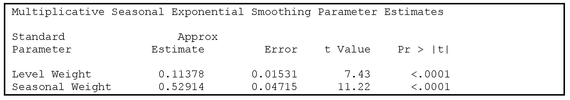
Figure 6.3 Forecasting the number of overnight stays by seasonal exponential smoothing in PROC ESM

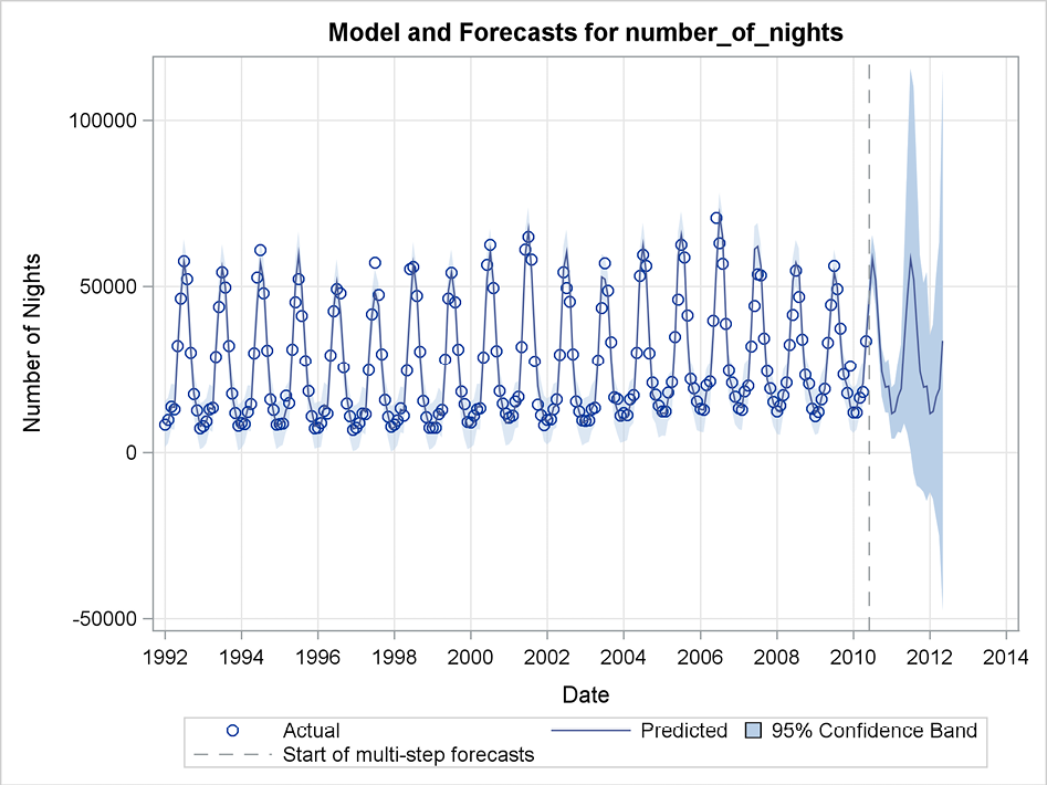
The forecasts simply form a continuation of the seasonal pattern in the observation period. As such they seem to be a realistic prediction of future values. The confidence limits in Figure 6.3 are broadening as the forecasting horizon increases. This is due to the fact that they are defined similarly to the definition in ARIMA models, including a difference operation. (See Section 7.5.) This means that forecast errors are cumulated for larger forecasting horizons, which is natural for time series that include trends in which departures from the trend seem to persist. For this actual series, no trend is present and steadily increasing forecast limits seem misleading. The next section presents a procedure call of PROC ESM, providing more realistic forecast limits.

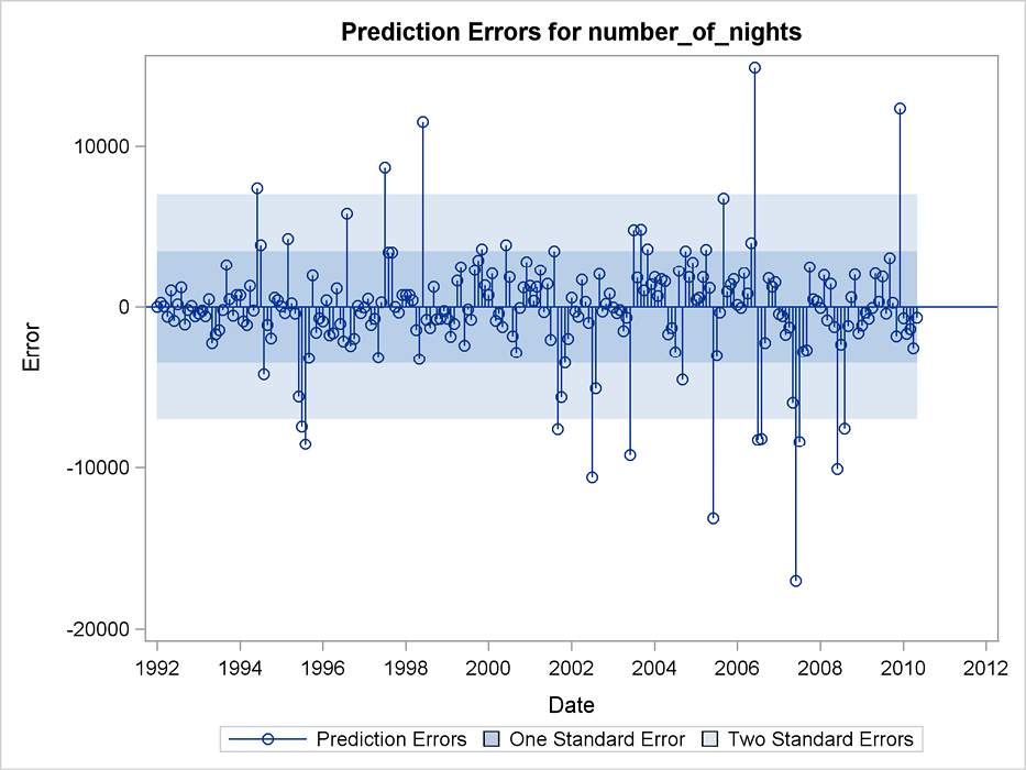
Figure 6.4 Residual plot for one-step-ahead forecasting of the number of overnight stays

6.4 Forecasting Using Additive Seasonal Exponential Smoothing with PROC ESM

PROC ESM also provides plots of the error structure in the observation period. See Figure 6.4, which is generated by Program 6.2. The overall picture is that no systematic variations in the errors occur in the signs of the errors but that a large number of marked outliers are present. As previously noted, such outliers are probably due to major scientific or political conferences with a large number of US participants.

This series has no trending behavior or shifting levels, and the seasonal variation is of the same absolute magnitude every year. This means that the seasonal component could be specified as additive instead of multiplicative because the idea of seasonality proportional to the level is irrelevant for this series. The additive version of exponential smoothing is obtained by the option method=addseasonal in the FORECAST statement, as shown in Program 6.3.

Program 6.3 An application of additive seasonal exponential smoothing using PROC ESM

ods graphics;
PROC ESM data=sasts.hotel print=estimates plot=all lead=24;
id date interval=month;
forecast number_of_nights/method=addseasonal;
run;
ods graphics off;

This additive version of the algorithm gives almost the same predictions as the multiplicative seasonal smoothing method applied in Section 6.3, but the confidence limits are narrower, as seen in Figure 6.5. The additive version is more appropriate when forecasting this series than the multiplicative version because this series has no trend at all. Methods that rely on a multiplicative seasonal structure are useful in series with clear level shifts, such as a price series where prices are rising due to inflation or a sales series without a well-defined level. The series in Section 6.6 is an example of a series for which a multiplicative structure is the right choice.

Figure 6.5 Forecasting the number of overnight stays using additive exponential smoothing in
PROC ESM

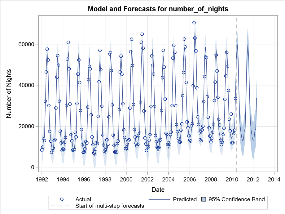
Figure 6.6 presents forecasts generated by the additive version of the Winters method for three years, with starting points every fourth year. The plot is drawn by a SAS macro, which applies PROC ESM several times. As seen in Figure 6.6, the additive method gives useful forecasts at least three years ahead because the seasonal structure in the series is fairly constant. Even if minor level shifts are seen, no systematic trend is present.

Figure 6.6 Forecasts of the number of overnight stays with no trend

6.5 Forecasting US Retail E-Commerce Using the Winters Method

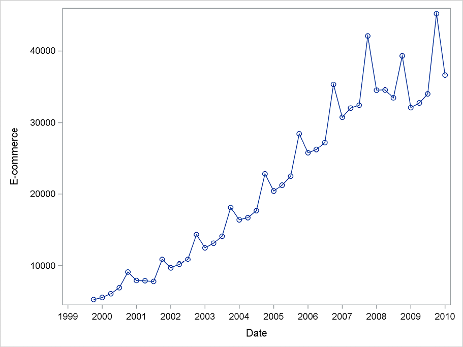
In this section, quarterly observations for the American retail sector are forecast. The focus is on the amount spent by consumers on e-commerce, using quarterly data. This data is published by the US Bureau of the Census as a series beginning the fourth quarter of 1999 and ending the first quarter 2010. First, the actual value of each year’s e-commerce is considered as the series shown in Figure 6.7. The seasonality is clear, with large sales in the fourth quarter of each year. The overall picture is a clear upward trend, which is natural due to inflation for a series denoted in dollars and the growing popularity of e-commerce in the American retail sector. The trend could also be linear in the observation period. However, since the third quarter of 2008, the trend has broken and retail sales have been constant, if not declining. This decline could be explained by the financial crisis. The seasonal pattern seems unstable during the crisis.

Figure 6.7 The value of US e-commerce

The code in Program 6.4 is used to forecast the e-commerce in 2008 and 2009 and assumes that no crisis had occurred. The last observation in the data set is for the first quarter of 2010. By specifying the option back=9 in the SAS code, the forecasts are generated using only observations up to the fourth quarter of 2007. The ID statement specifies the variable of the time index (date), and the option interval=quarter specifies the length of the seasonal period. The forecasts are calculated by using the Winters method, which includes both a linear trend and a multiplicative seasonal component. To use the Winters method, specify the option method=winters in the procedure statement, as in Program 6.4.

Program 6.4 An application of the Winters method in PROC ESM for forecasting the value of US e-commerce

ods graphics;
PROC ESM data=sasts.E_commerce print=estimates
plot=(MODELFORECASTS ERRORS) back=9 lead=20;
id date interval=quarter ;
forecast E_commerce/method=winters;
run;
ods graphics off;

Figure 6.8 Forecasting US e-commerce using the Winters method in PROC ESM from 2007

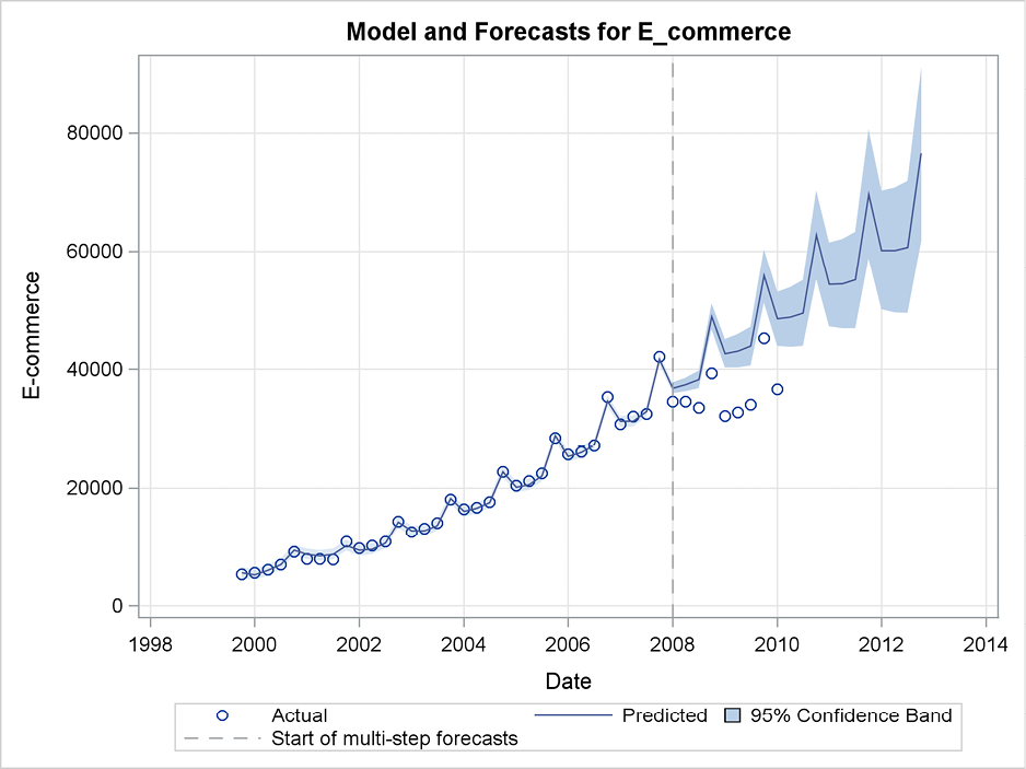
In the observation period for the years until 2007, Figure 6.8 shows that the peaks in the fourth quarters are fitted well by the predictions even if the absolute jump from third to fourth quarter is increasing. This result supports the choice of a multiplicative description of the seasonality, in contrast to the examples in Section 6.4.

The forecasts in Figure 6.8 are generated based on observations up to the fourth quarter of 2007. The forecasting period is 2008 and 2009, and for those years the forecasts are much higher than the actual observations of the sales. As previously suggested, these forecast errors can be seen as the impact of the financial crisis. In this case, the observed series is dominated by a clear linear trend, which is extracted by the Winters method and continued into the forecasting period. The forecasts are plotted for a long forecasting horizon, five years, by the option lead=20 in the SAS code. The functional form is dominated by the very strict seasonal component with the large retail sales in fourth quarter. An important feature of this forecasting method is that the seasonal component increases as the level of the retail sales increases, due to the trend component. For this data set, it is natural to expect the seasonality to be relative rather than absolute. For example, sales in the fourth quarter are 10% higher than the sales in the third quarter and not a fixed amount, such as one billion dollars higher independent of the level of the sales.

The forecast error variance in the observation period is rather small, and the forecast limits (which are by default 95%) are quite narrow. These narrow limits indicate that the forecasts are reliable. The confidence limits broaden for long-term forecasting, but in a way that seems reasonable. The poor performance of the forecasts is due to changing conditions, which are impossible to guess by using a technical procedure that uses historical data as the only information. Because departures from the one-period-ahead forecasts in the observation period are very small, the confidence limits are narrow and are in no way able to indicate an upcoming crisis in the near future.

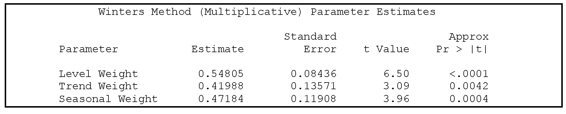
The parameters, which are written to the output window by the option print=estimates, are shown in Output 6.2. They are all around 0.5, which means that the calculation of the various components is performed giving almost equal weight to past values and to the most recent observation.

Output 6.2 Estimates for the parameters using the Winters method in PROC ESM

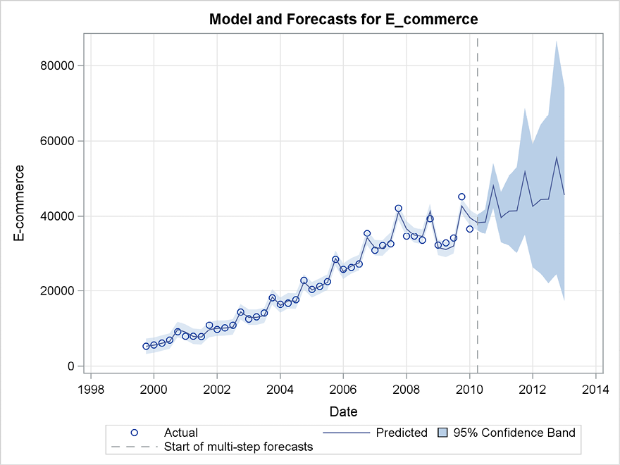
In Figure 6.9, the series is forecast using the last observed value, which is the first quarter of 2010, as a basis. This is done simply by deleting the option back=9 from the procedure statement. To some extent, the predictions during the crisis adapt to the new situation, so that the predictions almost equal the observed values. However, in the third and fourth quarters of 2009, the prediction errors are large. The forecast errors have a larger variance, and the confidence limits are for that reason much broader than in the plot where only information before the crisis was applied.

Predictions for the remaining quarters of 2010 and the following years are basically of the same form as the predictions based on 2007 where there is a strict seasonal pattern with an upward trend. Judging from these plots, the crisis caused a temporary pause in the upward trend in e-commerce. After this break, the upward trend is predicted to continue, which might well be the case. The effect of the broken trend is also seen by the prediction of the total value of e-commerce in 2012, which varies around $50,000M, compared with the predictions around $60,000M when 2007 is used as the basis.

Figure 6.9 Forecasting e-commerce from the last observation

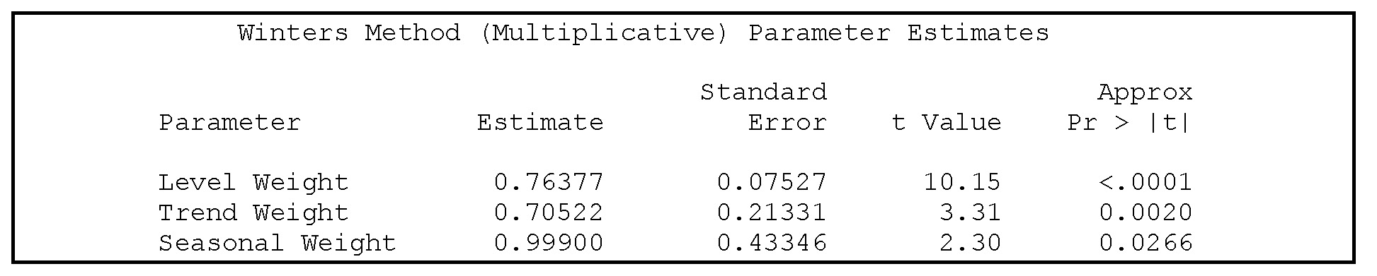
The parameters as estimated by PROC ESM using the whole time series as basis are shown in Output 6.3. They are much higher than when estimated using only observations before the crisis. This means that the calculation of the various components is performed giving less equal weight to past values and much more to the most recent observation. The weight parameter for the seasonal component is very large because the estimated value 0.999 is the maximal possible value for this parameter that is bounded by 1. This large value must be due to the volatile behavior during the crisis where the forecasting method tries to adapt to a new situation in which past experiences are of little use.

Output 6.3 Estimates by PROC ESM for the parameters of the Winters method

6.6 Forecasting the Relative Importance of E-Commerce by PROC ESM

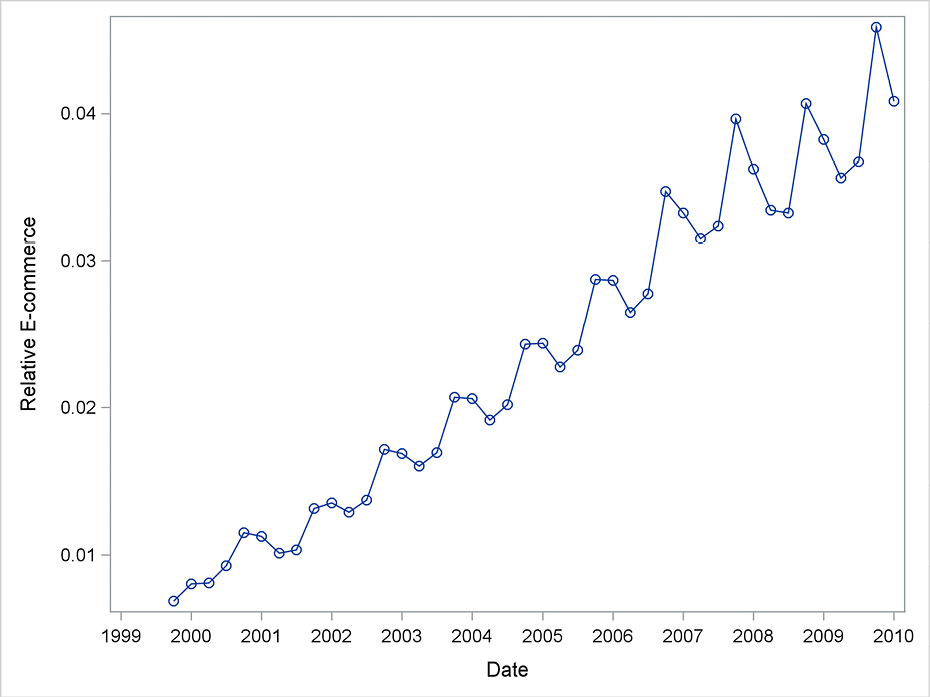
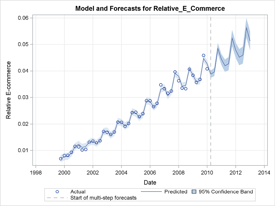
Next, the series of e-commerce relative to the total retail sales is forecast. This series is plotted in Figure 6.10. The main fact is that it increases steadily from around 1% in 2000 to approximately 4% in 2010. The relative importance of e-commerce seems to be unaffected by the financial crisis. The series is considered as a series of fractions and not as percents, because the series is transformed later in Section 6.7.

Figure 6.10 The relative importance of e-commerce

In this example, the seasonality in the curve formed by the forecasts in Figure 6.11 seems to change in the observation period from a rather smooth sinusoid to a jagged curve. This change in the seasonal component is reflected by the estimated parameters; see Output 6.4. The seasonal weight parameter is estimated to the maximum value 0.999. Then the algorithm gives total weight to the most recent observation of the seasonal component and neglects past values. The level parameter is also estimated using a high weight, which could be an indicator of instability in the level component. The weight in the trend estimation is as low as possible, 0.001, which indicates that the trend is completely fixed, as shown in the plot of the series.

Output 6.4 Estimates by PROC ESM for the parameters of the Winters method

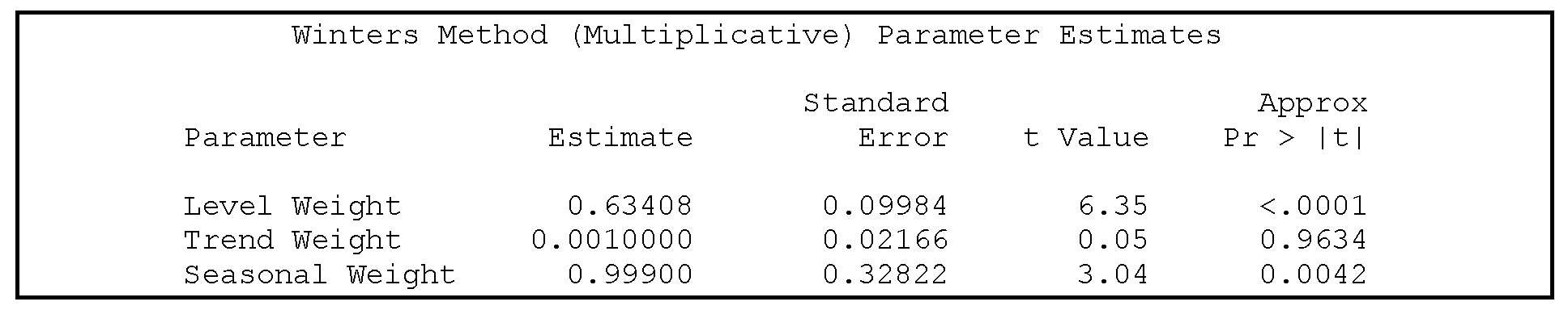
Figure 6.11 Forecasting the relative importance of e-commerce in the US retail sector

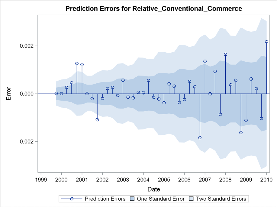
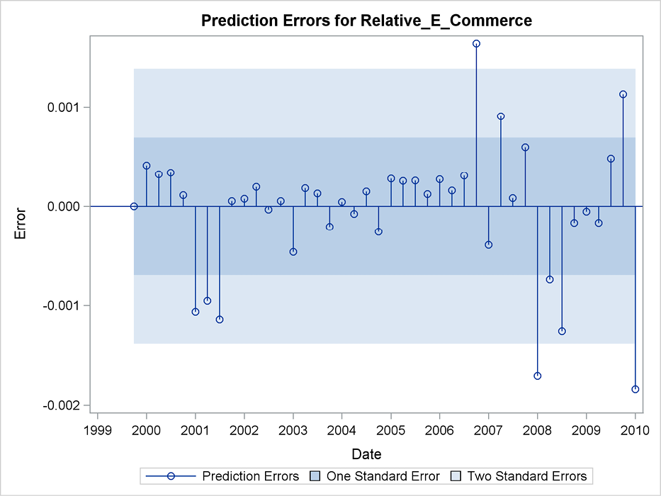
Although the fit and the plot of the forecast errors in the observation period, shown in Figure 6.12, indicate no signs of systematic behavior (which could be seen as obvious possibilities for improving the forecast), the plot discloses some heteroscedasticity in the residuals. The forecasts’ errors are numerically larger in the most recent years, which affects the assumptions underlying the calculation of confidence limits for these forecasts. In Section 6.7, this problem is discussed further and a solution by a natural transformation is applied.

Figure 6.12 Prediction errors for one-step-ahead forecasting of relative e-commerce

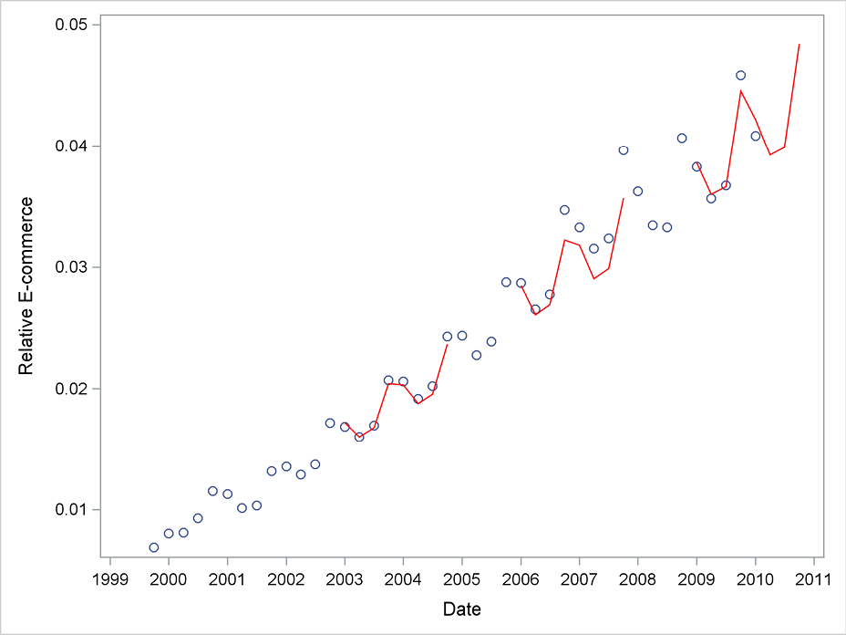
Even if the fit from a statistical viewpoint is doubtful because the variance is increasing, the forecasts are successful, as seen in Figure 6.13. The forecasts in Figure 6.13 are generated for a three-year horizon at three different starting times. Compared with the actual observations, the forecasts are precise. Moreover, the steadily increasing trend of the series is combined with a similar increase in the seasonal structure so that the amplitude of the seasonal fluctuations is much larger for the latest years than in the beginning of the observation period. This is clearly reflected because the forecasts fit the actual observations well.

This plot demonstrates that this forecasting method as applied by PROC ESM is very flexible and adaptable to changing situations. More standard statistical modeling typically relies on an assumption of a steady situation such as the formal definition of a stationary time series. For practical purposes, the flexibility offered by PROC ESM seems to make further statistical analyses superfluous.

Figure 6.13 Forecasts of the relative importance of e-commerce by the Winters method

6.7 Forecasting the Relative Importance of E-Commerce Using a Transformation in PROC ESM

It is obvious that a multiplicative formulation is preferred to an additive formulation for this data series. In this series, the seasonal variation increases in the years of observation during which the level of the series also increases, so the seasonality in the series is proportional to the level of the series. But in theory it is not obvious that the multiplicative formulation is optimal because this series, by the definition of a fraction, is bounded between 0 and 1. This could be a reason for abnormalities in the error plot, as mentioned in Section 6.6.

In the theory of marketing, a logistic curve is often applied when modeling market shares of new products. The logistic curve is bounded between 0 and 1. It is flat in the tails to 0 and 1, and the curve is steep in the middle for values of the fraction near one half. For this series, which is a fraction, the seasonality in the first years of the series (when the percentage of e-commerce to the total retail sales is low) will be increased by the transformation. However, the seasonality will be reduced for larger percentages, which leads to a more stable seasonal structure of the transformed series. This seasonal structure is easier to capture by the forecasting method.

Forecasting using the Winters method requires the series to be strictly positive. The logistic transformation results in negative transformed values if the fraction is less than one half. The logistic transformation cannot be applied directly in combination with the Winters method, which is the right choice for this series with a clear trend and seasonality. For this reason, the series is redefined and the series of conventional retail sales is applied. This series is simply defined as 1 minus the ratio of e-commerce to the total retail sales. This series decreases from 99% to 96% in the observation period. The series is analyzed by Program 6.5.

Program 6.5 Forecasting using the transformation facilities in PROC ESM

ods graphics;
PROC ESM data=sasts.E_commerce print=estimates
plot=(MODELFORECASTS ERRORS) lead=20 ;
id date interval=quarter ;
forecast Relative_Conventional_Commerce/ method=winters
transform=logistic alpha=0.2;
run;
ods graphics off;

In order to see the effect of the transformation, the forecasts are plotted in Figure 6.14 with a horizon of up to five years. The confidence limits are broad for such long horizons. Therefore, they are narrowed to an 80% confidence level by the option alpha=0.2.

Figure 6.14 Forecasting the percentage of conventional retails sales using a logistic transformation

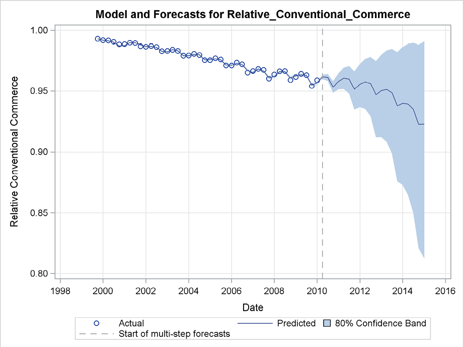
Figure 6.15 Histogram for residuals

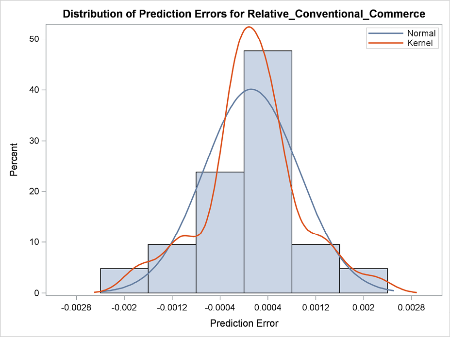
The error distribution is (as seen in Figure 6.15) skewed to the left, reflecting that the observed ratios are rather close to their upper limit of 1. By default, the predictions are calculated as the mean value in the distribution of the future values even if some transformation is applied. This could be misleading in situations with skewed error distribution as in this case where the share of conventional trade cannot exceed the number 1 but at least in theory could be much less than the mean value. For this reason, the actual prediction is not placed in the middle of the confidence interval but rather at a value that is too low. Another possibility offered by PROC ESM is to apply the median value rather than the mean value of the forecast distribution as the actual prediction. To apply the median value, specify the median option in the FORECAST statement. Comparing this method, which is used in Figure 6.16, with the expected value method in Figure 6.14 shows that the only difference between the plots is how the predictions are placed in the confidence region. When the median is applied as in Figure 6.16, the predictions are placed in the upper part of the region and the confidence level becomes skewed.

Figure 6.16 Forecasting a transformed series by the median

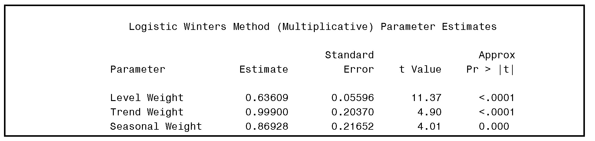
The estimated smoothing parameters are shown in Output 6.5. The weight parameter for the estimation of the trend practically equals 1, which means that the trend is calculated using the last observed value and rejects the information given by past values. To some extent, this conclusion holds true for the weight in the estimation of the seasonal component. However, these weight parameters are estimated with a fairly large standard deviation, so values much closer to 0 could work as well, according to the reported estimation results.

Output 6.5 Estimates by PROC ESM for the parameters of the Winters method

The transformation seems to be of no practical interest for short-term forecasting, but it is important for long-term forecasting. In this particular example, both the observed data series and common-sense intuition predict that the forecasts should include a clear decreasing tendency because the relative importance of e-commerce is believed to be increasing also in the forecasting period. When presenting forecasts over many years, the possibility of specifying asymmetrical confidence limits is useful. The forecaster can obtain reasonable limits and avoid negative values for strictly positive series. In this example, the forecaster can avoid ratios above 1.

In practice, this logistic transformation is seldom applied; the logarithmic transformation is used instead. This is easy to do by using the option transform=log, which at least leads to positive lower confidence limits so the counterintuitive negative confidence limits for long-term forecasting are avoided. In this example, one advantage is the non-constant confidence limits for the error terms, as seen in Figure 6.17. It is natural that this series, which is bounded above, is able to vary only moderately when it attains values close to the borders. This restriction occurs because relative conventional retail sales are very close to 1 for the first years of this observed series. As the share of conventional sales declines, the variation is allowed to increase, leading to an increasing confidence band for the forecast errors. See Figure 6.17.

Figure 6.17 Residuals with increasing confidence limits due to a transformation