
 7
7
t-Tests: Independent Samples and Paired Samples
Overview
This chapter describes the differences between the independent-samples t-test and the paired-samples t-test, and shows how to perform both types of analyses. An example of a research design is developed that provides data appropriate for each type of t-test. With respect to the independent-samples test, this chapter shows how to use JMP to determine whether the equal-variances or unequal-variances t-test is appropriate, and how to interpret the results. There are analyses of data for paired-samples research designs, with discussion of problems that can occur with paired data.
Introduction: Two Types of t-Tests
The Independent-Samples t-Test
Example: A Test of the Investment Model
Entering the Data into a JMP Data Table
General Outline for Summarizing Analysis Results
Example with Nonsignificant Differences
Examples of Paired-Samples Research Designs
Each Subject Is Exposed to Both Treatment Conditions
Problems with the Paired Samples Approach
When to Use the Paired Samples Approach
An Alternative Test of the Investment Model
Appendix: Assumptions Underlying the t-Test
Assumptions Underlying the Independent-Samples t-Test
Assumptions Underlying the Paired-Samples t-Test
Introduction: Two Types of t-Tests
A t-test is appropriate when an analysis involves a single nominal or ordinal predictor that assumes only two values (often called treatment conditions), and a single continuous response variable. A t-test helps you determine if there is a significant difference in mean response between the two conditions. There are two types of t-tests that are appropriate for different experimental designs.
First, the independent-samples t-test is appropriate if the observations obtained under one treatment condition are independent of (unrelated to) the observations obtained under the other treatment condition. For example, imagine you draw a random sample of subjects, and randomly assign each subject to either Condition 1 or Condition 2 in your experiment. You then determine scores on an attitude scale for subjects in both conditions, and use an independent-samples t-test to determine whether the mean attitude score is significantly higher for the subjects in Condition 1 than for the subjects in Condition 2. The independent-samples t-test is appropriate because the observations (attitude scores) in Condition 1 are unrelated to the observations in Condition 2. Condition 1 consists of one group of people, and Condition 2 consists of a different group of people who were not related to, or affected by, the people in Condition 1.
The second type of test is the paired-samples t-test. This statistic is appropriate if each observation in Condition 1 is paired in some meaningful way with a corresponding observation in Condition 2. There are a number of ways that this pairing happens. For example, imagine you draw a random sample of subjects and decide that each subject is to provide two attitude scores—one score after being exposed to Condition 1 and a second score after being exposed to Condition 2. You still have two samples of observations (the sample from Condition 1 and the sample from Condition 2), but the observations from the two samples are now related. If a given subject has a relatively high score on the attitude scale under Condition 1, that subject might also score relatively high under Condition 2. In analyzing the data, it makes sense to pair each subject’s scores from Condition 1 and Condition 2. Because of this pairing, a paired-samples t statistic is calculated differently than an independent-samples t statistic.
This chapter is divided into two major sections. The first deals with the independent-samples t-test, and the second deals with the paired-samples test. These sections describe additional examples of situations in which the two procedures might be appropriate.
Earlier, you read that a t-test is appropriate when the analysis involves a nominal or ordinal predictor variable and a continuous response. A number of additional assumptions should also be met for the test to be valid and these assumptions are summarized in an appendix at the end of this chapter. When these assumptions are violated, consider using a nonparametric statistic instead. See Basic Analysis and Graphing 2012), which is found on the Help menu, for examples of nonparametric statistics.
The Independent-Samples t-Test
Example: A Test of the Investment Model
The investment model of emotional commitment (Rusbult, 1980) illustrates the hypothesis tested by the independent-samples t-test. As discussed in earlier chapters, the investment model identifies a number of variables expected to affect a subject’s commitment to romantic relationships (as well as to some other types of relationships). Commitment can be defined as the subject’s intention to remain in the relationship and to maintain the relationship. One version of the investment model predicts that commitment will be affected by four variables—rewards, costs, investment size, and alternative value. These variables are defined as follows.
Rewards are the number of “good things” that the subject associates with the relationship (the positive aspects of the relationship).
Costs are the number of “bad things” or hardships associated with the relationship.
Investment Size is the amount of time and personal resources that the subject has “put into” the relationship.
Alternative Value is the attractiveness of the subject’s alternatives to the relationship (the attractiveness of alternative romantic partners).
At least four testable hypotheses can be derived from the investment model as it is described here.
- Rewards have a causal effect on commitment.
- Costs have a causal effect on commitment.
- Investment size has a causal effect on commitment.
- Alternative value has a causal effect on commitment.
This chapter focuses on testing only the first hypothesis: the prediction that the level of rewards affects commitment.
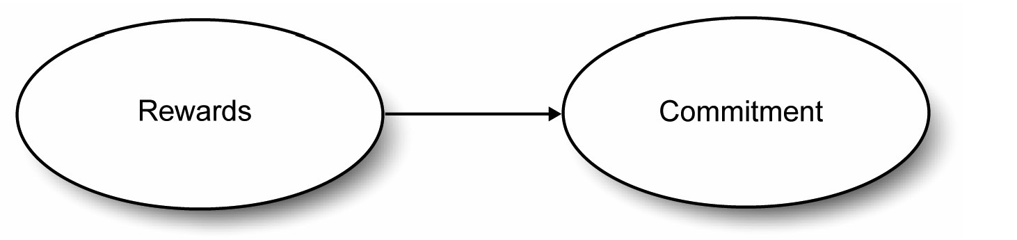
Rewards refer to the positive aspects of the relationship. Your relationship would score high on rewards if your partner were physically attractive, intelligent, kind, fun, rich, and so forth. Your relationship would score low on rewards if your partner were unattractive, unintelligent, unfeeling, dull, and so forth. It can be seen that the hypothesized relationship between rewards and commitment makes good intuitive sense: an increase in rewards should result in an increase in commitment. The predicted relationship between these variables is illustrated in Figure 7.1.
Figure 7.1: Hypothesized Causal Relationship between Rewards and Commitment
There are a number of ways that you could test the hypothesis that rewards have a causal effect on commitment. One approach involves an experimental procedure in which subjects are given a written description of different fictitious romantic partners and asked to rate their likely commitment to these partners. The descriptions are written so that a given fictitious partner can be described as a “high-reward” partner to one group of subjects, and as a “low-reward” partner to a second group of subjects. If the hypothesis about the relationship between rewards and commitment is correct, you expect to see higher commitment scores for the high-reward partner. This part of the chapter describes a fictitious study that utilizes just such a procedure, and tests the relevant null hypothesis using an independent-samples t-test.
The Commitment Study
Assume that you have drawn a sample of 20 subjects, and have randomly assigned 10 subjects to a high-reward condition and 10 to a low-reward condition. All subjects are given a packet of materials, and the following instructions appear on the first page:
In this study, you are asked to imagine that you are single and not involved in any romantic relationship. You will read descriptions of 10 different “partners” with whom you might be involved in a romantic relationship. For each description, imagine that you are involved in a romantic relationship with that person. Think about what it would be like to date that person, given his/her positive features, negative features, and other considerations. After you have thought about it, rate how committed you would be to maintaining your romantic relationship with that person. Each “partner” is described on a separate sheet of paper, and at the bottom of each sheet there are four items with which you can rate your commitment to that particular relationship.
The paragraph that described a given partner provides information about the extent to which the relationship with that person was rewarding and costly. It also provided information relevant to the investment size and alternative value associated with the relationship.
The Dependent Variable
The dependent variable in this study is the subject’s commitment to a specific romantic partner. It would be ideal if you could arrive at a single score that indicates how committed a given subject is to a given partner. High scores would reveal that the subject is highly committed to the partner, and low scores would indicate the opposite. This section describes one way that you could use rating scales to arrive at such a score.
At the bottom of the sheet that describes a given partner, the subject is provided with four items that use a 9-point Likert-type rating format. Participants are asked to respond to these items to indicate the strength of their commitment to the partner described on that page. The following items are used in making these ratings.
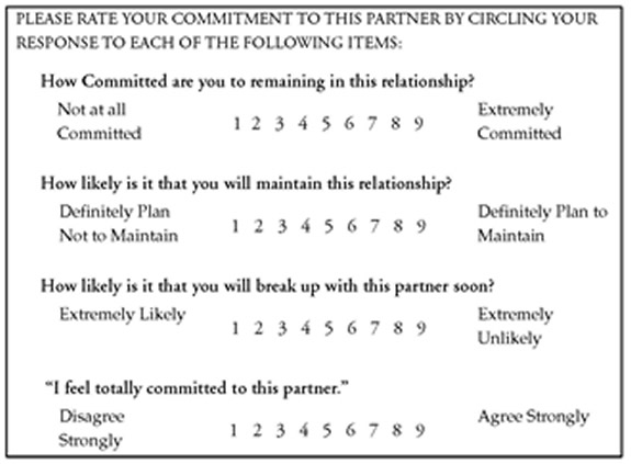
Notice that, with each of the preceding items, circling a higher response number (closer to “9”) reveals a higher level of commitment to the relationship. For a given partner, the subject’s responses to these four items were summed to arrive at a final commitment score for that partner. This score could range from a low of 4 (if the subject had circled the “1” on each item) to a high of 36 (if the subject had circled the “9” on each item). These scores serve as the dependent variable in your study.
Manipulating the Independent Variable
The independent variable in this study is “level of rewards associated with a specific romantic partner.” This independent variable was manipulated by varying the descriptions of the partners shown to the two treatment groups.
The first nine partner descriptions given to the high-reward group were identical to those given to the low-reward group. For partner 10, there was an important difference between the descriptions provided to the two groups. The sheet given to the high-reward group described a relationship with a relatively high level of rewards, but the one given to the low-reward group described a relationship with a relatively low level of rewards. Below is the description seen by subjects in the high-reward condition:
PARTNER 10: Imagine that you have been dating partner 10 for about a year, and you have put a great deal of time and effort into this relationship. There are not very many attractive members of the opposite sex where you live, so it would be difficult to replace this person with someone else. Partner 10 lives in the same neighborhood as you, so it is easy to see him or her as often as you like. This person enjoys the same recreational activities that you enjoy, and is also very good-looking.
Notice how the preceding description provides information relevant to the four investment model variables discussed earlier. The first sentence provides information dealing with investment size (“…you have put a great deal of time and effort into this relationship.”), and the second sentence deals with alternative value (“There are not very many attractive members of the opposite sex where you live....”). The third sentence indicates that this is a low-cost relationship because “…it is so easy to see him or her as often as you like.” In other words, there are no hardships associated with seeing this partner. If the descriptions said that the partner lives in a distant city, this would have been a high-cost relationship.
However, you are most interested in the last sentence because the last sentence describes the level of rewards associated with the relationship. The relevant sentence is “This person enjoys the same recreational activities that you enjoy, and is also very good-looking.” This statement establishes partner 10 as a high-reward partner for the subjects in the high-reward group.
In contrast, consider the description of partner 10 given to the low-reward group. Notice that it is identical to the description given to the high-reward group with regard to the first three sentences. The last sentence, however, deals with rewards, so this last sentence is different for the low-reward group. It describes a low-reward relationship:
PARTNER 10: Imagine that you have been dating partner 10 for about one year, and you have put a great deal of time and effort into this relationship. There are not very many attractive members of the opposite sex where you live, so it would be difficult to replace this person with someone else. Partner 10 lives in the same neighborhood as you, so it is easy to see him or her as often as you like. This person does not enjoy the same recreational activities that you enjoy, and is not very good-looking.
For this study, the vignette for partner 10 is the only scenario of interest. The analysis is only for the subjects’ ratings of their commitment to partner 10, and disregards their responses to the first nine partners. The first nine partners were included to give the subjects some practice at evaluating commitment before encountering item 10.
Also notice the logic behind these experimental procedures: both groups of subjects are treated in exactly the same way with respect to everything except the independent variable. Descriptions of the first nine partners are identical in the two groups. Even the description of partner 10 is identical with respect to everything except the level of rewards associated with the relationship. Therefore, if the subjects in the high-reward group are significantly more committed to partner 10 than the subjects in the low-reward group, you can be reasonably confident that it is the level of reward manipulation that affected their commitment ratings. It would be difficult to explain the results in any other way.
In summary, you began your investigation with 10 of 20 subjects randomly assigned to the high-reward condition and the other 10 subjects assigned to the low-reward condition. After the subjects complete their task, you disregard their responses to the first nine scenarios, but record their responses to partner 10 and analyze these responses.
Entering the Data into a JMP Data Table
Remember that an independent-samples t-test is appropriate for comparing two samples of observations. It allows you to determine whether there is a significant difference between the two samples with respect to the mean scores on their responses. More technically, it allows you to test the null hypothesis that, in the population, there is no difference between the two groups with respect to their mean scores on the response criterion. This section shows how to use the JMP Bivariate platform to test this null hypothesis for the current fictitious study.
The predictor variable in the study is “level of reward.” This variable can assume one of two values: subjects were either in the high-reward group or in the low-reward group. Because this variable simply codes group membership, you know that it is measured on a nominal scale. In coding the data, you can give subjects a score of “High” if they were in the high-reward condition and a score of “Low” if they were in the low-reward condition. You need a name for this variable, so call it Reward Group.
The response variable in this study is commitment, which is the subjects’ ratings of how committed they would be to a relationship with partner 10. When entering the data, the response is the sum of the rating numbers that have been circled by the subject in responding to partner 10. This variable can assume values from 4 through 36, and is a continuous numeric variable. Call this variable Commitment in the JMP data table.
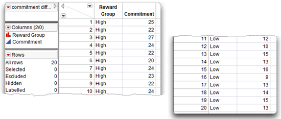
Figure 7.2 shows the JMP table, commitment difference.jmp, with this hypothetical data. Each line of data contains the group and the commitment response for one subject. Data from the 10 high-reward subjects were keyed first, followed by data from the 10 low-reward subjects. It is not necessary to enter the data sorted this way—data from low-reward and high-reward subjects could have been keyed in a random sequence.
Figure 7.2: Listing of the Commitment Difference JMP Data Table
Performing a t-Test in JMP
In the previous chapter, the Bivariate platform in JMP (Fit Y by X command) was used to look at measures of association between two continuous numeric variables. Now the Bivariate platform is used to test the relationship between a continuous numeric response variable and a nominal classification (predictor) variable.
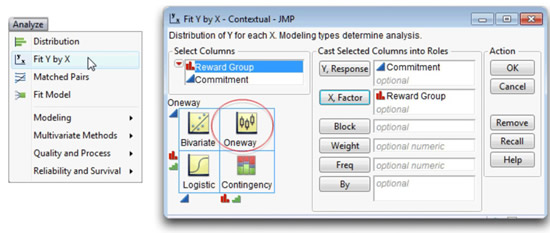
![]() To begin the analysis, choose Fit Y by X from the Analyze menu.
To begin the analysis, choose Fit Y by X from the Analyze menu.
![]() Select Commitment from the Select Columns list, and click the Y, Response button.
Select Commitment from the Select Columns list, and click the Y, Response button.
![]() Select Reward Group in the Select Columns list, and click the X, Factor button. Figure 7.3 shows the completed launch dialog.
Select Reward Group in the Select Columns list, and click the X, Factor button. Figure 7.3 shows the completed launch dialog.
Figure 7.3: Launch Dialog for Oneway Platform
Note: At any time, click the Help button to see help for the Oneway (Fit Y by X) platform. Or, choose the question mark (?) tool from the Tools menu or Tools palette, and click on the analysis results.
Results from the JMP Analysis
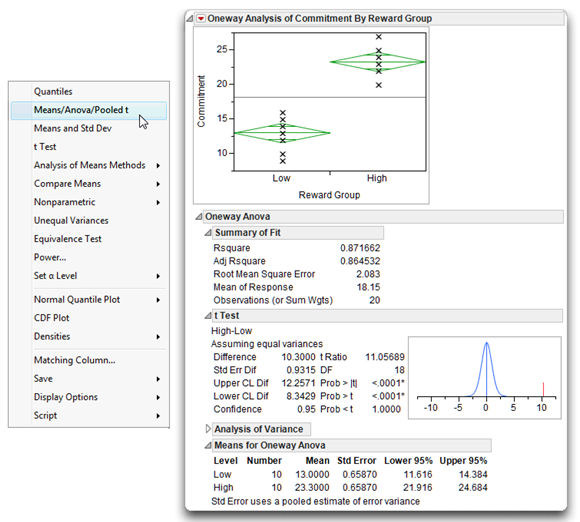
Click OK on the launch dialog to see the initial results. Figure 7.4 presents the results obtained from the JMP Bivariate platform for a continuous Y variable and a nominal or ordinal X variable. Initially, only the scatterplot of Commitment by Reward Group shows. To see a t-test, select Means/Anova/Pooled t from the menu found on the analysis title bar.
Notice that the title of the analysis is Oneway Analysis of Commitment By Reward Group. The Bivariate platform always performs a one-way analysis when the Y (dependent) variable is numeric and the X (independent or predictor) variable is nominal. When the X variable only has two levels, there are two types of independent t-test:
- The Means/Anova/Pooled t gives the t-test using the pooled standard error. This option also performs an analysis of variance, which is appropriate if the X variable has more than two levels.
- The t-Test menu option tests the difference between two independent groups assuming unequal variances, and therefore uses an unpooled standard error.
The analysis results are divided into sections. The scatterplot shows by default, with the Y variable (Commitment) on the Y axis and the predictor X variable (Reward Group) on the X axis.
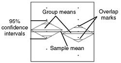
The Means/Anova/Pooled t option overlays means diamonds, illustrated above, on the groups in the scatterplot and appends several additional tables to the analysis results.
The means diamonds are a graphical illustration of the t-test. If the overlap marks do not vertically separate the groups, as in this example, the groups are probably not significantly different. The groups appear separated if there is vertical space between the top overlap mark of one diamond and the bottom overlap of the other diamond.
The t Test report gives the results of the t-test for the null hypothesis that the means of the two groups do not differ in the population. The following section describes a systematic approach for interpreting the t-test.
To change the markers in the scatterplot from the default small dots:
![]() Select all rows in the data table.
Select all rows in the data table.
![]() Choose the Markers command in the Rows main menu, and select a different marker from the markers palette.
Choose the Markers command in the Rows main menu, and select a different marker from the markers palette.
![]() Right-click in the scatterplot area and choose the Marker Size command. Select the size marker you want from the marker size palette.
Right-click in the scatterplot area and choose the Marker Size command. Select the size marker you want from the marker size palette.
Figure 7.4 Results of t-Test Analysis
Steps to Interpret the Results
Step1: Make sure that everything looks reasonable. As stated previously, the name of the nominal-level predictor variable appears on the X axis of the scatterplot, which shows the group values “Low” and “High.” Statistics in the Means for Oneway Anova table show the sample size (Number) for both high-reward and low-reward groups is 10. The mean Commitment score for the high-reward group is 23.3, and the mean score for the low-reward group is 13. The pooled standard error (Std Error) is 0.6587.
You should carefully review each of these figures to verify that they are within the expected range. For example, in this case you know there were no missing values so you want to verify that data for 10 subjects were observed for each group. In addition, you know that the Commitment variable was constructed such that it could assume possible values between 4 and 36. The observed group mean values are within these bounds, so there is no obvious evidence that an error was made keying the data.
Step 2: Review the t statistic and its associated probability value. The Means/Anova/Pooled t option in this example lets you review the equal-variances t statistics, as noted at the beginning of the t Test table. This t statistic assumes that the two samples have equal variances. In other words, the distribution of scores around the means for both samples is similar.
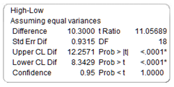
Descriptive statistics for the difference in the group means are listed on the left in the t Test table in Figure 7.4. The information of interest, on the right in this table, is the obtained t statistic, its corresponding degrees of freedom, and probability values for both one-tailed and two-tailed tests.
- The obtained t statistic (t ratio) is 11.057 (which is quite large).
- This t statistic is associated with 18 degrees of freedom.
- The next item, Prob > |t|, shows that the p-value associated with this t is less than 0.0001. This is the two-sided t-test, which tests the hypothesis that the true difference in means (difference in the population) is neither significantly greater than nor significantly less than the observed difference of 10.3.
But what does this p-value (p < 0.0001) really mean?
This p-value is the probability that you would obtain a t statistic as large as 11.057 or larger (in absolute magnitude) if the null hypothesis were true; that is, you would expect to observe an absolute t value greater than 11.056 by chance alone in only 1 of 10,000 samples if there were no difference in the population means. If this null hypothesis were true, you expect to obtain a t statistic close to zero.
You can state the null hypothesis tested in this study as follows:
“In the population, there is no difference between the low-reward group and the high-reward group with respect to their mean scores on the commitment variable.”
Symbolically, the null hypothesis can be represented
µ1 = µ2 or µ1 – µ 2 = 0
where µ1 is the mean commitment score for the population of people in the high-reward condition, and µ2 is the mean commitment score for the population of people in the low-reward condition.
Remember that, anytime you obtain a p-value less than 0.05, you reject the null hypothesis, and because your obtained p-value is so small in this case, you can reject the null hypothesis of no commitment difference between groups. You can therefore conclude that there is probably a difference in mean commitment in the population between people in the high-reward condition compared to those in the low-reward condition.
The two remaining items in the t Test table are the one-tailed probabilities for the observed t value, which tests not only that there is a difference, but also the direction of the difference.
- Prob > t is the probability (< 0.0001 in this example) that the difference in population group means is greater than the observed difference.
- Prob < t is the probability if (1.0000 in this example) that the difference in population group means is less than the observed difference.
Step 3: Review the graphic for the t-test. The plot to the right in the t Test table illustrates the t-test. The plot is for the t density with 18 degrees of freedom. The obtained t value shows as a red line on the plot. In this case, the t value of 11.057 falls far into the right tail of the distribution, making it easy to see why it is so unlikely that independent samples would produce a higher t than the one shown if the difference between the groups in the population is close to zero.
Step 4: Review the sample means. The significant t statistic indicates that the two populations are probably different from each other. The low-reward group has a mean score of 13.0 on the commitment scale, and the high-reward group has a mean score of 23.3. It is therefore clear that, as you expected, the high-reward group demonstrates a higher level of commitment compared to the low-reward group.
Step 5: Review the confidence interval for the difference between the means. A confidence interval extends from a lower confidence limit to an upper confidence limit. The t Test table in Figure 7.4 (also shown here) gives the upper confidence limit of the difference, Upper CL Dif, of 12.2571, and the lower confidence limit of the difference, Lower CL Dif, of 8.3429. Thus, the 95% confidence interval for the difference between means extends from 12.2571to 8.3429.
This means you can estimate with a 95% probability that in the population, the actual difference between the mean of the low-reward condition and the mean of the high-reward condition is somewhere between 12.2571 and 8.3429. Notice that this interval does not contain the value of zero (difference). This is consistent with your rejection of the null hypothesis, which states:
“In the population, there is no difference between the low-reward and high-reward groups with respect to their mean scores on the commitment variable.”
Step 6: Compute the index of effect size. In this example, the p-value is less than the standard criterion of .05 so you reject the null hypothesis. You know that there is a statistically significant difference between the observed commitment levels for the high-reward and low-reward conditions. But is it a relatively large difference? The null hypothesis test alone does not tell whether the difference is large or small. In fact, with very large samples you can obtain statistically significant results even if the difference is relatively trivial.
Because of this limitation of null hypothesis testing, many researchers now supplement statistics such as t-tests with measures of effect size. The exact definition of effect size varies depending on the type of analysis. For an independent samples t-test, effect size can be defined as the degree to which one sample mean differs from a second sample mean stated in terms of standard deviation units. That is, it is the absolute value of the difference between the group means divided by the pooled estimate of the population standard deviation.
The formula for effect size, denoted d, is
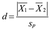
where
|
|
the observed mean of sample 1 (the participants in treatment condition 1) |
|
|
|
the observed mean of sample 2 (the participants in treatment condition 2) |
|
|
sp = |
the pooled estimate of the population standard deviation |
|
To compute the formula, use the sample means from the Means for Oneway Anova table, discussed previously. The estimate of the population standard deviation is the Root Mean Square Error found in the Summary of Fit table of the t-test analysis gives the pooled estimate of the population standard deviation (see Figure 7.4).
This result tells you that the sample mean for the low-reward condition differs from the sample mean for the high-reward condition by 4.9448 standard deviations. To determine whether this is a relatively large or small difference, you can consult the guidelines provided by Cohen (1992), which are shown in Table 7.1.
Table 7.1: Guidelines for Interpreting t-Test Effect Sizes
|
Effect Size |
Computed d Statistic |
|
Small effect |
d = 0.20 |
|
Medium effect |
d = 0.50 |
|
Large effect |
d = 0.80 |
The computed d statistic of 4.9448 for the commitment study is larger than the large-effect value in Table 7.1. This means that the differences between the low-reward and high-reward participants in commitment levels for partner 10 produced both a statistically significant and a very large effect.
General Outline for Summarizing Analysis Results
In performing an independent-samples t-test (and other analyses), the following format can be used to summarize the research problem and results:
A. Statement of the problem
B. Nature of the variables
C. Statistical test
D. Null hypothesis (H0)
E. Alternative hypothesis (H1)
F. Obtained statistic
G. Obtained probability p-value
H. Conclusion regarding the null hypothesis
I. Sample means and confidence interval of the difference
J. Effect size
K. Figure representing the results
L. Formal description of results for a paper
The following is a summary of the preceding example analysis according to this format.
A. Statement of the problem
The purpose of this study was to determine whether there is a difference between people in a high-reward relationship and those in a low-reward relationship with respect to their mean commitment to the relationship.
B. Nature of the variables
This analysis involved two variables. The predictor variable was level of rewards, which was measured on a nominal scale and could assume two values: a low-reward condition (coded as “Low”) and a high-reward condition (coded as “High”). The response variable was commitment, which was a numeric continuous variable constructed from responses to a survey with values ranging from 4 through 36.
C. Statistical test
Independent-samples t-test, assuming equal variances.
D. Null hypothesis (H0)
µ1 = µ 2. In the population, there is no difference between people in a high-reward relationship and those in a low-reward relationship with respect to their mean levels of commitment.
E. Alternative hypothesis (H1)
µ 1 µ 2. In the population, there is a difference between people in a high-reward relationship and those in a low-reward relationship with respect to their mean levels of commitment.
F. Obtained statistic
t = 11.057.
G. Obtained probability p-value
p < .0001.
H. Conclusion regarding the null hypothesis
Reject the null hypothesis.
I. Sample means and confidence interval of the difference
The difference between the high-reward and the low-reward means was 23.3 – 13 = 10.3. The 95% confidence interval for this difference extended from 8.3429 to 12.2571.
J. Effect size
d = 4.94 (large effect size).
K. Figure representing the results
To produce the chart shown here:
![]() Choose Chart command from the Graph menu.
Choose Chart command from the Graph menu.
![]() Select Reward Group as X. Select Commitment and choose Mean from the statistics menu as Y, and then click OK.
Select Reward Group as X. Select Commitment and choose Mean from the statistics menu as Y, and then click OK.
![]() From the red triangle menu on the Chart title bar, choose Label Options > Show Labels.
From the red triangle menu on the Chart title bar, choose Label Options > Show Labels.
L. Formal description of results for a paper
Most chapters in this book show you how to summarize the results of an analysis in a way that would be appropriate if you were preparing a paper to be submitted for publication in a scholarly research journal. These summaries generally follow the format recommended in the Publication Manual of the American Psychological Association (2009), which is required by many journals in the social sciences.
Here is an example of how the current results could be summarized according to this format:
Results were analyzed using an independent-samples t-test. This analysis revealed a significant difference between the two groups: t (18) = 11.05689; p <0.0001. The sample means are displayed with a bar chart, which illustrates that subjects in the high-reward condition scored significantly higher on commitment than did subjects in the low-reward condition (for high-reward group, Mean = 23.30, SD = 1.95; for low-reward group, Mean = 13.00, SD = 2.21). The observed difference between means was 10.30, and the 95% confidence interval for the difference between means extended from 8.34 to 12.26. The effect size was computed as d = 4.94. According to Cohen’s (1992) guidelines for t-tests, this represents a large effect.
Example with Nonsignificant Differences
Researchers do not always obtain significant results when performing investigations such as the one described in the previous section. This section repeats the analyses, this time using fictitious data that result in a nonsignificant t-test. The conventions for summarizing nonsignificant results are then presented.
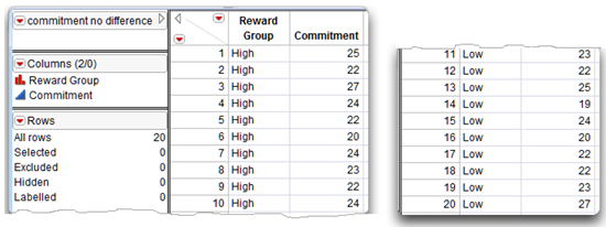
The data table for the following example is commitment no difference.jmp. The data have been modified so that the two groups do not differ significantly on mean levels of commitment. Figure 7.5 shows this JMP table. Simply “eyeballing” the data reveals that similar commitment scores seem to be displayed by subjects in the two conditions. Nonetheless, a formal statistical test is required to determine whether significant differences exist.
Figure 7.5: Example Data for Nonsignificant t-Test
Proceed as before.
![]() Use Analyze > Fit Y by X (see Figure 7.3).
Use Analyze > Fit Y by X (see Figure 7.3).
![]() When the results appear, select the Means/Anova/Pooled t from the menu on the analysis title bar (see Figure 7.4).
When the results appear, select the Means/Anova/Pooled t from the menu on the analysis title bar (see Figure 7.4).
![]() Also select the Means and Std Dev option, as illustrated in Figure 7.6. This option shows the pooled standard deviation used to compute t values in this example and in the previous example.
Also select the Means and Std Dev option, as illustrated in Figure 7.6. This option shows the pooled standard deviation used to compute t values in this example and in the previous example.
Figure 7.6: Results of Analysis with Nonsignificant t-Test
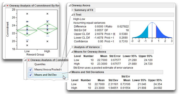
The t Test table in Figure 7.6 shows the t statistic (assuming equal variances) to be small at 0.627 and p-value for this t statistic is large at 0.5380. Because this p-value is greater than the standard cutoff of 0.05, you can say that the t statistic is not significant. These results mean that you don’t reject the null hypothesis of equal population means on commitment. In other words, you conclude that there is not a significant difference between mean levels of commitment in the two samples.
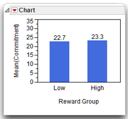
This analysis shows the Means and Std Deviations table for the data, which gives the Std Dev and Std Error Mean for each level of the Commitment variable. Note that, as before, the Std Error value in the Means for Oneway Anova table is the same for both levels because the pooled error is used in the t-test computations. The mean commitment score is 23.3 for the high-reward group and 22.7 for the low-reward group. The t Test table shows the difference between the means is 0.6 with lower confidence limit of –1.4078 and upper confidence limit of 2.6078. Notice that this interval includes zero, which is consistent with your finding that the difference between means is not significant (or, say the difference is not significantly different than zero).
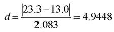
Compute the effect size of the difference as the difference between the means divided by the estimate of the standard deviation of the population (Root Mean Square Error in the Summary of Fit table):
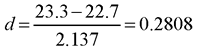
Thus the index of effect size for the current analysis is 0.2802. According to Cohen’s guidelines in Table 7.1, this value falls between a small and medium effect.
For this analysis, the statistical interpretation format appears as follows. This is the same study as shown previously so you can complete items A through E in the same way.
F. Obtained statistic
t = 0.6278.
G. Obtained probability p-value
p= 0.5380 .
H. Conclusion regarding the null hypothesis
Fail to reject the null hypothesis.
I. Sample means and confidence interval of the difference
The difference between the high-reward and the low-reward means was 23.3 – 22.7 = 0.6. The 95% confidence interval for this difference extended from
–1.4078 to 2.6078.
J. Effect size
d = 0.2808 (small to medium effect size)
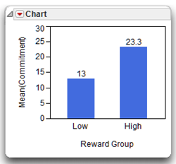
K. Figure representing the results
To produce the chart shown here:
![]() Choose Chart command in the Graph menu.
Choose Chart command in the Graph menu.
![]() Select Reward Group as X. Select Commitment and choose Mean from the statistic menu as Y, then click OK.
Select Reward Group as X. Select Commitment and choose Mean from the statistic menu as Y, then click OK.
![]() Then, from the red triangle menu on the Chart title bar, choose Label Options > Show Labels.
Then, from the red triangle menu on the Chart title bar, choose Label Options > Show Labels.
L. Formal description of results for a paper
The following is an example of a formal description of the results.
Results were analyzed using an independent-samples t-test. This analysis failed to reveal a significant difference between the two groups, t(18) = 0.628 giving p = 0.538. The bar chart of the sample means illustrate that subjects in the high-reward condition demonstrated scores on commitment that were similar to those shown by subjects in the low-reward condition (for high-reward group, Mean = 23.30, SD = 1.95; for low-reward group, Mean = 22.70, SD = 2.31). The observed difference between means was 0.6 and the 95% confidence interval for the difference between means extended from –1.41 to 2.61. The effect size was computed as d = 0.28. According to Cohen’s (1992) guidelines for t-tests, this represents a small to medium effect.
The Paired-Samples t-Test
The paired-samples t-test (sometimes called the correlated-samples t-test or matched-samples t-test) is similar to the independent-samples test in that both procedures compare two samples of observations, and determine whether the mean of one sample is significantly differs from than the mean of the other. With the independent-samples procedure, the two groups of scores are completely independent. That is, an observation in one sample is not related to any observation in the other sample. Independence is achieved in experimental research by drawing a sample of subjects and randomly assigning each subject to either condition 1 or condition 2. Because each subject contributes data under only one condition, the two samples are empirically independent.
In contrast, each score in one sample of the paired-samples procedure is paired in some meaningful way with a score in the other sample. There are several ways that this can happen. The following examples illustrate some of the most common paired situations.
Examples of Paired-Samples Research Designs
Be aware that the following fictitious studies illustrate paired sample designs, but might not represent sound research methodology from the perspective of internal or external validity. Problems with some of these designs are reviewed later.
Each Subject Is Exposed to Both Treatment Conditions
Earlier sections described an experiment in which level of reward was manipulated to see how it affected subjects’ level of commitment to a romantic relationship. The study required that each subject review 10 people and rate commitment to each fictitious romantic partner. The dependent variable is the rated amount of commitment the subjects displayed toward partner 10. The independent variable is manipulated by varying the description of partner 10: subjects in the “high-reward” condition read that partner 10 had positive attributes, while subjects in the “low-reward” condition read that partner 10 did not have these attributes. This study is an independent-samples study because each subject was assigned to either a high-reward condition or a low-reward condition (but no subject was ever assigned to both conditions).
You can modify this (fictitious) investigation so that it follows a paired-samples research design by conducting the study with only one group of subjects instead of two groups. Each subject rates partner 10 twice, once after reading the low-reward version of partner 10, and a second time after reading the high-reward version of partner 10.
It would be appropriate to analyze the data resulting from such a study using the paired-samples t-test because it is possible to meaningfully pair observations under the both conditions. For example, subject 1’s rating of partner 10 under the low-reward condition can be paired with his or her rating of partner 10 under the high-reward condition, subject 2’s rating of partner 10 under the low-reward condition could be paired with his or her rating of partner 10 under the high-reward condition, and so forth. Table 7.2 shows how the resulting data could be arranged in tabular form.
Remember that the dependent variable is still the commitment ratings for partner 10. Subject 1 (John) has two scores on this dependent variable—a score of 11 obtained in the low-reward condition, and a score of 19 obtained in the high-reward condition. John’s score in the low-reward condition is paired with his score from the high-reward condition. The same is true for the remaining participants.
Table 7.2: Fictitious Data from a Study Using a Paired Samples Procedures
|
Low-Reward Condition |
High-Reward Condition |
|
|
John |
11 |
19 |
|
Mary |
9 |
22 |
|
Tim |
10 |
23 |
|
Susan |
9 |
18 |
|
Maria |
12 |
21 |
|
Fred |
12 |
25 |
|
Frank |
17 |
22 |
|
Edie |
15 |
25 |
|
Jack |
14 |
24 |
|
Shirley |
19 |
31 |
Matching Subjects
The preceding study used a type of repeated measures approach. There is only one sample of participants, and repeated measurements on the dependent variable (commitment) are taken from each participant. That is, each person contributes one score under the low-reward condition and a second score under the high-reward condition.
A different approach could have used a type of matching procedure. With a matching procedure, a given participant provides data under only one experimental condition. However, each person is matched with certain conditions to a different person who provides data under the other experimental condition:
- The participants are matched on some variable that is expected to be related to the dependent variable.
- The matching is done prior to the manipulation of the independent variable.
For example, imagine that it is possible to administer an emotionality scale to subjects. Further, prior research has shown that scores on this scale are strongly correlated with scores on romantic commitment (the dependent variable in your study). You could administer this emotionality scale to 20 participants, and use their scores on that scale to match them. That is, you could place them in pairs according to their similarity on the emotionality scale.
Now suppose scores on the emotionality scale range from a low of 100 to a high of 500. Assume that John scores 111 on this scale, and William scores 112. Because their scores are very similar, you pair them together, and they become subject pair 1. Tim scores 150 on this scale, and Fred scores 149. Because their scores are very similar, you also pair them together as subject pair 2. Table 7.3 shows how you could arrange these fictitious pairs of subjects.
Within a subject pair, one participant is randomly assigned to the low-reward condition, and one is assigned to the high-reward condition. Assume that, for each of the pairs in Table 7.3, the person listed first was randomly assigned to the low-reward condition, and the person listed second was assigned to the high-reward condition. The study then proceeds in the usual way, with subjects rating the various paper people.
Table 7.3: Fictitious Data from a Study Using a Matching Procedure
(continued)
|
Commitment Ratings of Partner 10 |
|||
|
|
Low-Reward Condition |
High-Reward Condition |
|
|
Subject pair 1 |
8 |
19 |
|
|
Subject pair 2 |
9 |
21 |
|
|
Subject pair 3 |
10 |
21 |
|
|
Subject pair 4 |
10 |
23 |
|
|
Subject pair 5 |
11 |
24 |
|
|
Subject pair 6 |
13 |
26 |
|
|
Subject pair 7 |
14 |
27 |
|
|
Subject pair 8 |
14 |
28 |
|
|
Subject pair 9 |
16 |
30 |
|
|
Subject pair 10 |
18 |
32 |
|
Table 7.3 shows that, for Subject pair 1, John gave a commitment score of 8 to partner 10 in the low-reward condition; William gave a commitment score of 19 to partner 10 in the high-reward condition. When analyzing the data, you pair John’s score on the commitment variable with William’s score on commitment. The same will be true for the remaining subject pairs. A later section shows how to analyze the data using JMP.
Remember that subjects are placed together in pairs on the basis of some matching variable before the independent variable is manipulated. The subjects are not placed together in pairs on the basis of their scores on the dependent variable. In the present case, subjects are paired based on the similarity of their scores on the emotionality scale that was administered previously. Later, the independent variable is manipulated and the subjects’ commitment scores are recorded. Although they are not paired on the basis of their scores on the dependent variable, you hope that their scores on the dependent variable will be correlated. There is more discussion on this in a later section.
Take Pretest and Posttest Measures
Consider now a different type of research problem. Assume that an educator believes that taking a foreign language course causes an improvement in critical thinking skills among college students. To test the hypothesis, the educator administers a test of critical thinking skills to a single group of college students at two points in time:
- A pretest is administered at the beginning of the semester (prior to taking the language course).
- A posttest is administered at the end of the semester (after completing the course).
The data obtained from the two test administrations appear in Table 7.4.
Table 7.4: Fictitious Data from Study Using a Pretest-Posttest Procedure
|
Scores on Test of |
||
|
Subject |
Pretest |
Posttest |
|
John |
34 |
55 |
|
Mary |
35 |
49 |
|
Tim |
39 |
59 |
|
Susan |
41 |
63 |
|
Maria |
43 |
62 |
|
Fred |
44 |
68 |
|
Frank |
44 |
69 |
|
Edie |
52 |
72 |
|
Jack |
55 |
75 |
|
Shirley |
57 |
78 |
You can analyze these data using the paired-samples t-test because it is meaningful to pair the same subject’s pretest and posttest scores. When the data are analyzed, the results indicate whether there was a significant increase in critical thinking scores over the course of the semester.
Problems with the Paired Samples Approach
Some of the studies described in the preceding section use fairly weak experimental designs. This means that, even if you had conducted the studies, you might not have been able to draw firm conclusions from the results because alternative explanations could be offered for those results.
Order Effects
Consider the first investigation that exposes each subject to both the low-reward version of partner 10 as well as the high-reward version of partner 10. If you designed this study poorly, it might suffer from confoundings that make it impossible to interpret the results. For example, suppose you design the study so that each subject rates the low-reward version first and the high-reward version second? If you then analyze the data and find that higher commitment ratings were observed for the high-reward condition, you would not know whether to attribute this finding to the manipulation of the independent variable (level of rewards) or to order effects. Order effects are the possibility that the order in which the treatments were presented influenced scores on the dependent variable. In this example it is possible that subjects tend to give higher ratings to partners that are rated later in serial order. If this is the case, the higher ratings observed for the high-reward partner may simply reflect such an order effect.
Alternative Explanations
The third study, which investigated the effects of a language course on critical thinking skills, also displays a weak experimental design. The single-group pretest-posttest design assumes you administered the test of critical thinking skills to the students at the beginning and again at the end of the semester. It further assumes that you observe a significant increase in their skills over this period as would be consistent with your hypothesis that the foreign language course helps develop critical thinking skills.
However, there are other reasonable explanations for the findings. Perhaps the improvement was simply due to the process of maturation—changes that naturally take place as people age. Perhaps the change is due to the general effects of being in college, independent of the effects of the foreign language
course. Because of the weak design used in this study, you will probably never be able to draw firm conclusions about what was really responsible for the students’ improvement.
This is not to argue that researchers should never obtain the type of data that can be analyzed using the paired-samples t-test. For example, the second study described previously (the matching procedure) was reasonably sound and might have provided interpretable results. The point here is that research involving paired-samples must be designed very carefully to avoid the sorts of problems discussed here. You can deal with most of these difficulties through the appropriate use of counterbalancing, control groups, and other strategies. The problems inherent in repeated measures and matching designs, along with the procedures that can be used to handle these problems, are discussed in Chapter 11, One-Way anova with One Repeated-Measures Factor, and Chapter 12, Factorial ANOVA with Repeated-Measures Factors and Between-Subjects Factors.
When to Use the Paired Samples Approach
When conducting a study with only two treatment conditions, you often have the choice of using either the independent-samples approach or the paired-samples approach. One of the most important considerations is the extent to which the paired-samples analysis can result in a more sensitive test. That is, to what extent is the paired-samples approach more likely to detect significant differences when they actually do exist?
It is important to understand that the paired-samples t-test has one important weakness in regard to sensitivity—it has only half the degrees of freedom as the equivalent independent-samples test. Because the paired-samples approach has fewer degrees of freedom, it must display a larger t-value than the independent-samples t-test to attain statistical significance.
However, under the right circumstances, the paired-samples approach results in a smaller standard error of the mean (the denominator in the formula used to compute the t statistic, and a smaller standard error usually results in a more sensitive test. The exception is that the paired-samples approach results in a smaller standard error only if scores on the two sets of observations are positively correlated with one another. This concept is easiest to understand with reference to the pretest-posttest study shown in Table 7.3.
Notice that scores on the pretest appear to be positively correlated with scores on the posttest. That is, subjects who obtained relatively low scores on the pretest (such as John) also tended to obtain relatively low scores on the posttest. Similarly, subjects who obtained relatively high scores on the pretest (such as Shirley) also tended to obtain relatively high scores on the posttest. This shows that although the subjects might have displayed a general improvement in critical thinking skills over the course of the semester, their ranking relative to one another remained relatively constant. The subjects with the lowest scores at the beginning of the term still tended to have the lowest scores at the end of the term.
The situation described here is the type of situation that makes the paired-samples t-test the optimal procedure. Because pretest scores are correlated with posttest scores, the paired-samples approach should yield a fairly sensitive test.
The same logic applies to the other studies described previously. For example, look at the values in Table 7.2, from the study in which subjects were assigned to pairs based on matching criteria. There appears to be a correlation between scores obtained in the low-reward condition and those obtained in the high-reward condition. This could be because subjects were first placed into pairs based on the similarity of their scores on the emotionality scale, and the emotionality scale is predictive of how subjects respond to the commitment scale. For example, both John and William (pair 1) display relatively low scores on commitment, presumably because they both scored low on the emotionality scale that was initially used to match them. Similarly, both George and Dave (subject pair 10) scored relatively high on commitment, presumably because they both scored high on emotionality.
This illustrates why it is so important to select relevant matching variables when using a matching procedure. There is a correlation between the two commitment variables above because (presumably) emotionality is related to commitment. If you had instead assigned subjects to pairs based on some variable that is not related to commitment (such as subject shoe size), the two commitment variables would not be correlated, and the paired-samples t-test would not provide a more sensitive test. Under those circumstances, you achieve more power by instead using the independent-samples t-test and capitalizing on the greater degrees of freedom.
An Alternative Test of the Investment Model
The remainder of this chapter shows how to use JMP to perform paired-sample
t-tests, and describes how to interpret the results. The first example is based on the fictitious study that investigates the effect of levels of reward on commitment to a romantic relationship. The investigation included 10 subjects, and each subject rated partner 10 after reviewing the high-reward version of partner 10, and again after reviewing the low-reward version. Figure 7.7 shows the data keyed into a JMP data table called commitment paired.jmp.
Figure 7.7: Paired Commitment Data
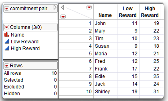
Notice in the JMP table that the data are arranged exactly as they were presented in Table 7.2. The two score variables list commitment ratings obtained when subjects reviewed the low-reward version of partner 10 (Low Reward), and when they reviewed the high-reward version of partner 10 (High Reward).
It is easy to do a paired t-test in JMP.
![]() Choose the Matched Pairs command from the Analyze menu.
Choose the Matched Pairs command from the Analyze menu.
![]() When the launch dialog appears, select the Low Reward and the High Reward variables (the set of paired responses) and click the Y, Paired Response button to enter them as the paired variables to be analyzed.
When the launch dialog appears, select the Low Reward and the High Reward variables (the set of paired responses) and click the Y, Paired Response button to enter them as the paired variables to be analyzed.
![]() Click OK to see the results in Figure 7.8.
Click OK to see the results in Figure 7.8.
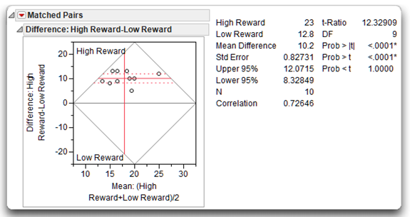
Figure 7.8: Results from Paired t Analysis
Interpret the Paired t Plot
Like most JMP analyses, the results start with a graphic representation of the analysis. The illustration here describes the paired t-test plot, using y1 and y2 as the paired variables. The vertical axis is the difference between the group means, with a zero line that represents zero difference between means.
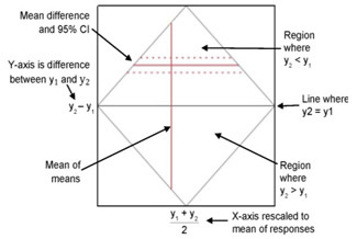
If the dotted 95% confidence lines (around the plotted difference) also encompass the zero reference, then you visually conclude there is no difference between group means. In Figure 7.8, the mean difference and its confidence lines are far away from the zero reference so you can visually conclude there is a difference between groups.
Note: The diamond-shaped rectangle on the plot results from the Reference Frame option found in the red triangle menu on the Matched Pairs title bar.
Interpret the Paired t Statistics
The Matched Pairs report lists basic summary statistics. You can see that the mean commitment score in the low-reward condition is 12.8, and the mean commitment score in the high-reward condition is 23.0. Subjects displayed higher levels of commitment for the high-reward version of partner 10.
Also note in the Matched Pairs report that the lower 95% confidence limit (Lower95%) is 8.3265, and the upper limit (Upper95%) is 12.0715. This lets you estimate with 95% probability that the actual difference between the mean of the low-reward condition and the mean of the high-reward condition (in the population) is between these two confidence limits. Also, as shown in the plot above, this interval does not contain zero, which indicates you will be able to reject the null hypotheses. If there was no difference between group means, you expect the confidence interval to include zero (a difference score of zero).
Note that the Mean Difference is 10.2, and the standard error of the difference is 0.82731. The paired t analysis determines whether this mean difference is significantly different from zero. Given the way that this variable was created, a positive value on this difference indicates that, on the average, scores for High Reward tended to be higher than scores for Low Reward. The direction of this difference is consistent with your prediction that higher rewards are associated with greater levels of commitment.
Next, review the results of the t-test to determine whether this mean difference score is significantly different from zero. The t statistic in a paired-samples t-test is computed using the following formula:
t = Md / SEd
where
|
Md = |
the mean difference score |
|
SEd = |
the standard error of the mean for the difference scores (the standard deviation of the sampling distribution of means of difference scores). |
This t-value in this example is obtained by dividing the mean difference score of 10.2 by the standard error of the difference (0.82731 shown in the results table), giving t = 12.32909. Your hypothesis is one-sided—you expect high reward groups to have significantly higher commitment scores. Therefore, the probability of getting a greater positive t-value shows as Prob > t and is less than 0.0001. This p-value is much lower than the standard cutoff of 0.05, which indicates that the mean difference score of 10.2 is significantly greater than zero. Therefore you can reject the null hypothesis that the population difference score was zero, and conclude that the mean commitment score of 23.0 observed with the high-reward version of partner 10 is significantly higher than the mean score of 12.8 observed with low-reward version of partner 10. In other words, you tentatively conclude that the level of reward manipulation had an effect on rated commitment.
The degrees of freedom associated with this t-test are N –1, where N is the number of pairs of observations in the study. This is analogous to saying that N is equal to the number of difference scores that are analyzed. If the study involves taking repeated measures from a single sample of subjects, N will be equal to the number of subjects. However, if the study involves two sets of subjects who are matched to form subject pairs, N will be equal to the number of subject pairs, which is one-half the total number of subjects.
The present study involved taking repeated measures from a single sample of 10 participants. Therefore, N = 10 in this study, and the degrees of freedom are
10 – 1 = 9, as in the t-test results shown in Figure 7.8.
Effect Size of the Result
The previous example in this chapter defined effect size, d, as the degree to which a mean score obtained under one condition differs from the mean score obtained under a second condition. For the paired t-test, the d statistic is computed by dividing the difference between the means by the estimated standard deviation of the population of difference scores. That is,
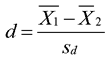
where
|
|
the observed mean of sample 1 (the participants in treatment condition 1) |
|
|
the observed mean of sample 2 (the participants in treatment condition 2) |
|
sd = |
the estimated standard deviation of the population of difference scores |
The Paired t Test report does not show sd but it is computed as the standard error (Std Err), shown in the t Test Analysis report, multiplied by the square root of the sample size (N). That is,
sd = (Std Err * √N) = (0.82731 * √10) = (0.82731 * 3.162) = 2.616
Then d is computed,
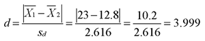
Thus, the obtained index of effect size for the current study is 3.999, which means the commitment score under the low-reward condition differs from the mean commitment score under the high-reward condition by almost four standard deviations. To determine whether this is a large or small difference, refer to the guidelines provided by Cohen (1992), which are shown in Table 7.1. Your obtained d statistic of 3.999 is much larger than the “large effect” value of 0.80. This means that the manipulation in your study produced a very large effect.
Summarize the Results of the Analysis
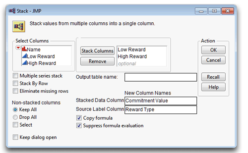
One way to produce a summary bar chart is to stack the paired commitment scores in the two reward columns into a single column, and use the Chart platform to plot the means of the reward groups. The example in Chapter 3, “Working with JMP Data,” uses this paired data to show how to stack columns. With the Commitment Paired data table active,
![]() Choose Stack from the Tables menu.
Choose Stack from the Tables menu.
![]() Select the Low Reward and High Reward variables and click Add to add them to the Stack Columns list, as shown in Figure 7.9.
Select the Low Reward and High Reward variables and click Add to add them to the Stack Columns list, as shown in Figure 7.9.
![]() Uncheck the Stack by Row box on the dialog, which is checked by default.
Uncheck the Stack by Row box on the dialog, which is checked by default.
Figure 7.9: Stack Dialog to Stack Commitment Scores into a Single Column
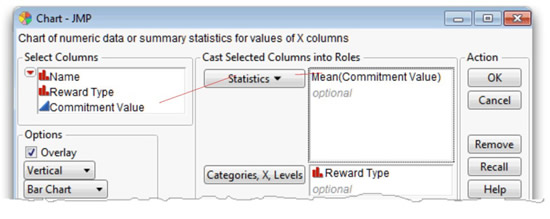
![]() Choose Graph > Chart, complete the Chart dialog as in Figure 7.10, and then click OK.
Choose Graph > Chart, complete the Chart dialog as in Figure 7.10, and then click OK.
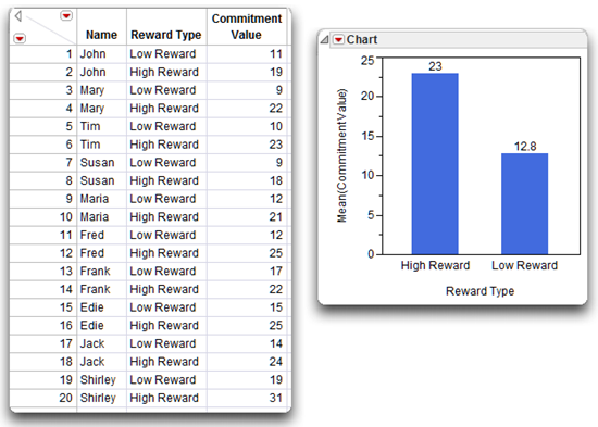
You should now see the data table shown on the left in Figure 7.11. This data table with stacked columns is now in the same form as the one shown previously in Figure 7.5, used to illustrate the independent samples t-test.
Figure 7.10: Completed Chart Dialog to Chart Mean Commitment Scores
![]() From the red triangle menu on the Chart title bar, choose Label Options > Show Labels to show the mean commitment value on each bar.
From the red triangle menu on the Chart title bar, choose Label Options > Show Labels to show the mean commitment value on each bar.
![]() Experiment with other options on the Chart menu to see what they do.
Experiment with other options on the Chart menu to see what they do.
Figure 7.11: Stacked Table and Bar Chart of Means
You can summarize the results of the present analysis following the same format used with the independent group’s t-test, as presented earlier in this chapter.
Results were analyzed using a paired-samples t-test. This analysis revealed a significant difference between mean levels of commitment observed in the two conditions, t (9) = 12.32 and p < 0.0001. The sample means are displayed as a bar chart in Figure 7.11, which shows that mean commitment scores appear significantly higher in the high-reward condition (mean = 23) than in the low-reward condition (mean = 12.8). The observed difference between these scores was 10.2, and the 95% confidence interval for the difference extended from 8.3285 to 12.0715. The effect size was computed as d = 3.999. According to Cohen’s (1992) guidelines for t-tests, this represents a very large effect.
A Pretest-Posttest Study
A previous section presented the hypothesis that taking a foreign language course leads to an improvement in critical thinking among college students. To test this hypothesis, assume that you conducted a study in which a single group of college students took a test of critical thinking skills both before and after completing a semester-long foreign language course. The first administration of the test constituted the study’s pretest, and the second administration constituted the posttest. The JMP data table, languagetext.jmp, which is shown on the left in Figure 7.12, has the results of the study.
Analyze the data using the same approach shown in the previous example.
![]() Choose the Matched Pairs command from the Analyze menu.
Choose the Matched Pairs command from the Analyze menu.
![]() When the launch dialog appears, select Pretest (each participant’s score on the pretest) and Posttest (each participant’s score on the posttest), and click the Y, Paired Response button to enter them as the pair of variables to be analyzed.
When the launch dialog appears, select Pretest (each participant’s score on the pretest) and Posttest (each participant’s score on the posttest), and click the Y, Paired Response button to enter them as the pair of variables to be analyzed.
![]() Click OK to see the results in Figure 7.12.
Click OK to see the results in Figure 7.12.
Figure 7.12: Data for Pretest and Posttest Language Scores
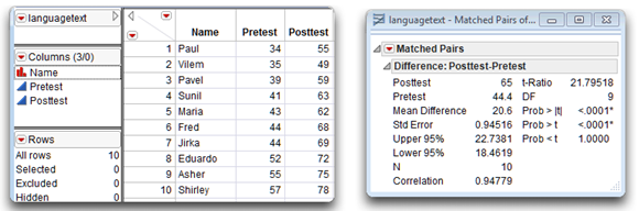
The positive mean difference in score (Posttest–Pretest) is consistent with the hypothesis that taking a foreign language course causes an improvement in critical thinking. You can interpret the results in the same manner as the previous example. This analysis reveals a significant difference between mean levels of pretest scores and posttest scores, with
t(9) = 21.7951 and p < 0.0001.
Summary
The t-test is one of the most commonly used statistics in the social sciences, in part because some of the simplest investigations involve the comparison of just two treatment conditions. When an investigation involves more than two conditions, however, the t-test is no longer appropriate, and you usually replace it with the F test obtained from an analysis of variance (ANOVA). The simplest ANOVA procedure—the one-way ANOVA with one between-subjects factor—is the topic of the next chapter.
Appendix: Assumptions Underlying the t-Test
Assumptions Underlying the Independent-Samples t-Test
Level of measurement
The response variable should be assessed on an interval- or ratio-level of measurement. The predictor variable should be a nominal-level variable that must include two categories (groups).
Independent observations
A given observation should not be dependent on any other observation in either group. In an experiment, you normally achieve this by drawing a random sample and randomly assigning each subject to only one of the two treatment conditions. This assumption would be violated if a given subject contributed scores on the response variable under both treatment conditions. The independence assumption is also violated when one subject’s behavior influences another subject’s behavior within the same condition. The texts discussed in this chapter rely on the assumption of independent observations. If this assumption is not met, inferences about the population (results of hypothesis tests) can be misleading or incorrect.
Random sampling
Scores on the response variable should represent a random sample drawn from the populations of interest.
Normal distributions
Each sample should be drawn from a normally distributed population. If each sample contains over 30 subjects, the test is robust against moderate departures from normality.
Homogeneity of variance
To use the equal-variances t-test, you should draw the samples from populations with equal variances on the response variable. If the null hypothesis of equal population variances is rejected, you should use the unequal-variances t-test.
Assumptions Underlying the Paired-Samples t-Test
Level of measurement
The response variable should be assessed on an interval-l or ratiolevel of measurement. The predictor variable should be a nominal-level variable that must include just two categories.
Paired observations
A given observation appearing in one condition must be paired in some meaningful way with a corresponding observation appearing in the other condition. You can accomplish this by having each subject contribute one score under condition 1, and a separate score under condition 2. Observations can also be paired by using a matching procedure to create the sample.
Independent observations
A given subject’s score in one condition should not be affected by any other subject’s score in either of the two conditions. It is acceptable for a given subject’s score in one condition to be dependent upon his or her own score in the other condition. This is another way of saying that it is acceptable for subjects’ scores in condition 1 to be correlated with their scores in condition 2.
Random sampling
Subjects contributing data should represent a random sample drawn from the populations of interest.
Normal distribution for difference scores
The differences in paired scores should be normally distributed. These difference scores are usually created by beginning with a given subject’s score on the dependent variable obtained under one treatment condition and subtracting from it that subject’s score on the dependent variable obtained under the other treatment condition. It is not necessary that the individual dependent variables be normally distributed, as long as the distribution of difference scores is normally distributed.
Homogeneity of variance
The populations represented by the two conditions should have equal variances on the response criterion.
References
American Psychological Association. 2009. Publication Manual of the American Psychological Association, 6th Edition. Washington, D.C: American Psychological Association.
Cohen, J. 1992. “A Power Primer.” Psychological Bulletin, 112, 155–159.
Rusbult, C. E. 1980. “Commitment and Satisfaction in Romantic Associations: A Test of the Investment Model.” Journal of Experimental Social Psychology, 16, 172–186.
SAS Institute Inc. 2012. JMP Basic Analysis and Graphing. Cary, NC: SAS Institute Inc.