
 8
8
One-Way ANOVA with One Between-Subjects Factor
Overview
In this chapter you learn how to enter data and use JMP to perform a one-way analysis of variance. This chapter focuses on the between-subjects design, in which each subject is exposed to only one condition under the independent variable. The use of a multiple comparison procedure (Tukey’s HSD test) is described, and guidelines for summarizing the results of the analysis in tables and text are provided.
Introduction: Basics of One-Way ANOVA Between-Subjects Design
Between-Subjects Designs versus Repeated-Measures Designs
Multiple Comparison Procedures
Statistical Significance versus Magnitude of the Treatment Effect
Example with Significant Differences between Experimental Conditions
Using JMP for Analysis of Variance
Ordering Values in Analysis Results
Steps to Interpret the Results
Summarize the Results of the Analysis
Example with Nonsignificant Differences between Experimental Conditions
Summarizing the Results of the Analysis with Nonsignificant Results
Understanding the Meaning of the F Statistic
Appendix: Assumptions Underlying One-Way ANOVA with One Between-Subjects Factor
Introduction: Basics of One-Way ANOVA Between-Subjects Design
One-way analysis of variance (ANOVA) is appropriate when an analysis involves:
- a single nominal or ordinal predictor (independent) variable that can assume two or more values
- a single continuous numeric response variable
In Chapter 7, “t-Tests: Independent Samples and Paired Samples,” you learned about the independent samples t-test, which you can use to determine whether there is a significant difference between two groups of subjects with respect to their scores on a continuous numeric response variable. But what if you are conducting a study in which you need to compare more than just two groups? In that situation, it is often appropriate to analyze your data using a one-way ANOVA.
The analysis that this chapter describes is called one-way ANOVA because you use it to analyze data from studies in which there is only one predictor variable (or independent variable). In contrast, Chapter 9, “Factorial ANOVA with Two Between-Subjects Factors,” presents a statistical procedure that is appropriate for studies with two predictor variables.
The Aggression Study
To illustrate a situation for which one-way ANOVA might be appropriate, imagine you are conducting research on aggression in children. Assume that a review of prior research has led you to believe that consuming sugar causes children to behave more aggressively. You therefore wish to conduct a study that will test the following hypothesis:
“The amount of sugar consumed by eight-year-old children increases the levels of aggression that they subsequently display.”
To test your hypothesis, you conduct an investigation in which each child in a group of 60 children is randomly assigned to one of three treatment conditions:
- 20 children are assigned to the “0 grams of sugar” treatment condition.
- 20 children are assigned to the “20 grams of sugar” treatment condition.
- 20 children are assigned to the “40 grams of sugar” treatment condition.
The independent variable in the study is the amount of sugar consumed. You manipulate this variable by controlling the amount of sugar that is contained in the lunch each child receives. In this way, you ensure that the children in the “0 grams of sugar” group are actually consuming 0 grams of sugar, that the children in the “20 grams of sugar” group are actually consuming 20 grams, and so forth.
The dependent variable in the study is the level of aggression displayed by each child. To measure this variable, a pair of observers watches each child for a set period of time each day after lunch. These observers tabulate the number of aggressive acts performed by each child during this time. The total number of aggressive acts performed by a child over a 2-week period serves as that child’s score on the dependent response variable. You can see that the data from this investigation are appropriate for a one-way ANOVAbecause
- the study involves a single predictor variable which is measured on a nominal scale (amount of sugar consumed)
- the predictor variable assumes more than two values (the 0-gram group, the 20-gram group, and the 40-gram group)
- the study involves a single response variable (number of aggressive acts) that is treated as a continuous numeric variable
Between-Subjects Designs versus Repeated-Measures Designs
The research design that this chapter discusses is referred to as a between-subjects design because each subject appears in only one group, and comparisons are made between different groups of subjects. For example, in the experiment just described, a given subject is assigned to just one treatment condition (such as the 20-gram group), and provides data on the dependent variable from only that specific treatment condition.
A distinction, therefore, is made between a between-subjects design and a repeated-measures design. With a repeated-measures design, a given subject provides data under each of the treatment conditions used in the study. It is called a repeated-measures design because each subject provides repeated measurements on the dependent variable.
A one-way ANOVA with one between-subjects factor is directly comparable to the independent-samples t-test from the last chapter. The difference is that you can use a t-test to compare just two groups, but you use a one-way ANOVA to compare two or more groups. In the same way, a one-way ANOVA with one repeated-measures factor is very similar to the paired-samples t-test from the last chapter. Again, the main difference is that you use a t-test to analyze data from just two treatment conditions but use a repeated-measures ANOVA with data from two or more treatment conditions. The repeated-measures ANOVA is covered in Chapter 11, “One-Way ANOVA with One Repeated-Measures Factor.”
Multiple Comparison Procedures
When you analyze data from an experiment with a between-subjects ANOVA, you can state the null hypothesis like this:
“In the population, there is no difference between the various treatment conditions with respect to their mean scores on the dependent variable.”
For example, for the preceding study on aggression, you might state a null hypothesis that, in the population, there is no difference between the 0-gram group, the 20-gram group, and the 40-gram group with respect to the mean number of aggressive acts performed. This null hypothesis could be represented symbolically as
µ1 = µ2 = µ3
where µ1 represents the mean level of aggression shown by the 0-gram group, µ2 represents mean aggression shown by the 20-gram group, and µ3 represents mean aggression shown by the 40-gram group.
When you analyze your data, JMP tests the null hypothesis by computing an F statistic. If the F statistic is sufficiently large (and the p-value associated with the F statistic is sufficiently small), you can reject the null hypothesis. In rejecting the null hypotheses, you tentatively conclude that, in the population, at least one of the three treatment conditions differs from at least one other treatment condition on the measure of aggression.
However, this leads to a problem: which pairs of treatment groups are significantly different from one another? Perhaps the 0-gram group is different from the 40-gram group, but is not different from the 20-gram group. Perhaps the 20-gram group is different from the 40-gram group, but is not different from the 0-gram group. Perhaps all three groups are significantly different from one another.
Faced with this problem, researchers routinely rely on multiple comparison procedures. Multiple comparison procedures are statistical tests used in studies with more than two groups to help determine which pairs of groups are significantly different from one another. JMP offers several different multiple comparison procedures:
- a simple t-test to compare each pair of groups
- Hsu’s MCB, which compares each group to the best (one group you choose)
- Tukey’s HSD (Honestly Significant Difference), which compares each pair of groups with an adjusted probability
- Dunnett’s test to compare each group to a control group you specify
This chapter shows how to request and interpret Tukey’s studentized range test, sometimes called Tukey’s HSD test (for Honestly Significant Difference). The Tukey test is especially useful when the various treatment groups in the study have unequal numbers of subjects, which is often the case.
Statistical Significance versus Magnitude of the Treatment Effect
This chapter also discusses the R2 statistic from the results of an analysis of variance. In an ANOVA, R2 represents the proportion or percent of variance in the response that is accounted for or explained by variability in the predictor variable. In a true experiment, you can view R2 as an index of the magnitude of the treatment effect. It is a measure of the strength of the relationship between the predictor and the response. Values of R2 range from 0 through 1. Values closer to 0 indicate a weak relationship between the predictor and response, and values closer to 1 indicate a stronger relationship.
For example, assume that you conduct the preceding study on aggression in children. If your independent variable (amount of sugar consumed by the children) has a very weak effect on the level of aggression displayed by the children, R2 will be a small value, perhaps 0.02 or 0.04. On the other hand, if your independent variable has a very strong effect on their level of aggression, R2 will be a larger value, perhaps 0.20 or 0.40. Exactly how large R2 must be to be considered “large” depends on a number of factors that are beyond the scope of this chapter.
It is good practice to report R2 or some other measure of the magnitude of the effect in a published paper because researchers like to draw a distinction between results that are merely statistically significant versus those that are truly meaningful. The problem is that very often researchers obtain results that are statistically significant, but not meaningful in terms of the magnitude of the treatment effect. This is especially likely to happen when conducting research with a very large sample. When the sample is very large (say, several hundred subjects), you might obtain results that are statistically significant even though your independent variable has a very weak effect on the dependent variable (this is because many statistical tests become very sensitive to minor group differences when the sample is large).
For example, imagine that you conduct the preceding aggression study with 500 children in the 0-gram group, 500 children in the 20-gram group, and 500 children in the 40-gram group. It is possible that you would analyze your data with a one-way ANOVA, and obtain an F value that is significant at p < 0.05. Normally, this might lead you to rejoice. But imagine that you then calculate R2 for this effect, and learn that R2 is only 0.03. This means that only 3% of the variance in aggression is accounted for by the amount of sugar consumed. Obviously, your manipulation has had a very weak effect. Even though your independent variable is statistically significant, most researchers would argue that it does not account for a meaningful amount of variance in children’s aggression.
This is why it is helpful to always provide a measure of the magnitude of the treatment effect (such as R2) along with your test of statistical significance. In this way, your readers will always be able to assess whether your results are truly meaningful in terms of the strength of the relationship between the predictor variable and the response.
Example with Significant Differences between Experimental Conditions
To illustrate one-way ANOVA, imagine that you replicate the study that investigated the effect of rewards on commitment in romantic relationships, which was described previously in Chapter 7. However, in this investigation you use three experimental conditions instead of the two experimental conditions described previously.
Recall that the preceding chapter hypothesized that the rewards people experience in a romantic relationship have a causal effect on their commitment to those relationships. You tested this prediction by conducting an experiment with 20 participants. The participants were asked to read the descriptions of 10 potential romantic partners. For each partner, the subjects imagined what it would be like to date this person, and rated how committed they would be to a relationship with that person. For the first 9 partners, every subject saw exactly the same description. However, there were some important differences with respect to partner 10:
- Half of the subjects had been assigned to a high-reward condition, and these subjects were told that partner 10 “...enjoys the same recreational activities that you enjoy, and is very good looking.”
- The other half of the subjects were assigned to the low-reward condition, and were told that partner 10 “...does not enjoy the same recreational activities that you enjoy, and is not very good looking.”
You are now going to repeat this experiment using the same procedure as before, but this time add a third experimental condition called the mixed-reward condition. Here is the description of partner 10 to be read by subjects assigned to the mixed reward group.
PARTNER 10: Imagine that you have been dating partner 10 for about 1 year, and you have put a great deal of time and effort into this relationship. There are not very many attractive members of the opposite sex where you live, so it would be difficult to replace this person with someone else. Partner 10 lives in the same neighborhood as you, so it is easy to be together as often as you like. Sometimes this person seems to enjoy the same recreational activities that you enjoy, and sometimes does not. Sometimes partner 10 seems to be very good looking, and sometimes is not.
Notice that the first three sentences of the preceding description are identical to the descriptions read by subjects in the low-reward and high-reward conditions in the previous experiment. These three sentences deal with investment size, alternative value, and costs, respectively. However, the last two sentences deal with rewards, and they are different from the sentences dealing with rewards in the other two conditions. In this mixed-reward condition, partner 10 is portrayed as being something of a mixed bag. Sometimes this partner is rewarding to be around, and sometimes not.
The purpose of this new study is to determine how the mixed-reward version of partner 10 will be rated. Will this version be rated more positively than the version provided in the low-reward condition? Will it be rated more negatively than the version provided in the high-reward condition?
To conduct this study, you begin with a total sample of 18 subjects. You randomly assign 6 to the high-reward condition, and they read the high-reward version of partner 10, as it was described in the chapter on t-tests. You randomly assign 6 subjects to the low-reward condition, and they read the low-reward version of partner 10. Finally, you randomly assign 6 subjects to the mixed-reward condition, and they read the mixed-reward version just presented. As was the case in the previous investigation, you analyze subjects’ ratings of how committed they would be to a relationship with partner 10 (and ignore their ratings of the other 9 partners).
You can see that this study is appropriate for analysis with a one-way ANOVA, between-subjects design because this study
- involves a single predictor variable assessed on a nominal scale (type of rewards)
- involves a single response variable assessed on an interval scale (rated commitment)
- involves three treatment conditions (low-reward, mixed-reward, and high-reward), making it inappropriate for analysis with an independent-groups t-test
The following section shows how to analyze fictitious data using JMP to do a one-way ANOVA with one between-subjects factor.
Using JMP for Analysis of Variance
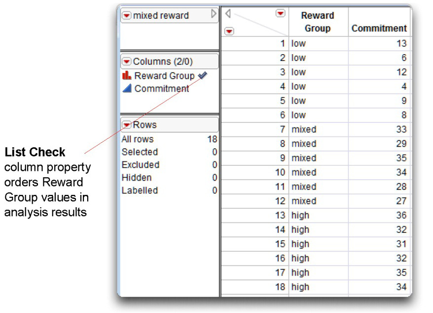
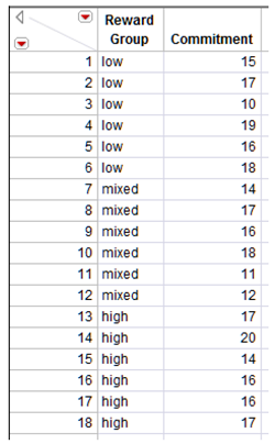
The data table used in this study is called mixed reward.jmp (see Figure 8.1). There is one observation for each subject. The predictor variable is type of reward, called Reward Group, with values “low,” “mixed,” and “high.” The response variable is Commitment. It is the subjects’ rating of how committed they would be to a relationship with partner 10. The value of this variable is based on the sum of subject responses to four questionnaire items described in the last chapter and can assume values from 4 through 36. It is a numeric variable with a continuous modeling type.
Figure 8.1: Mixed-Reward Data Table
Ordering Values in Analysis Results
The downward arrow icon to the right of the Reward Group name in the Columns panel indicates that column is assigned the List Check column property. The List Check property lets you specify the order you want variable values to appear in analysis results. In this example, you want to see Reward Group values listed in the order “low,” “mixed,” and “high.” Unless otherwise specified, values in reports appear in alphabetic order.
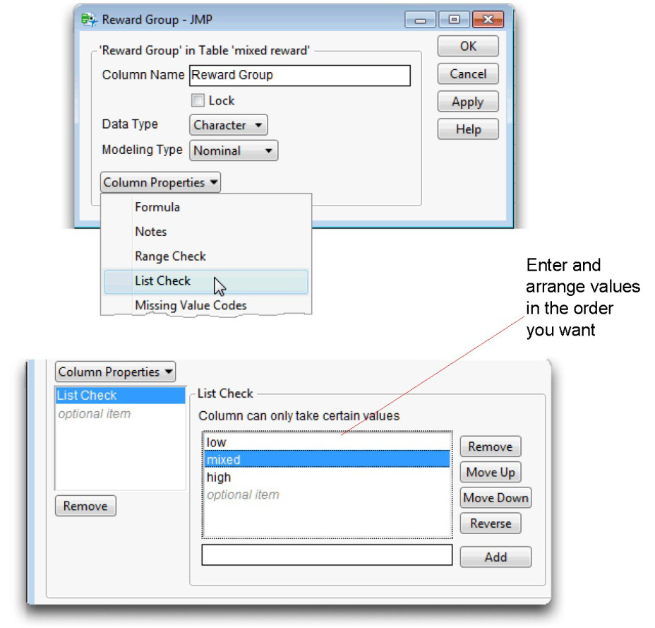
One way to order values in analysis results is to use the Column Info dialog and assign a special property to the column called List Check. To do this,
![]() Right-click in the Reward Group column name area or on the column name in the Columns panel, and select Column Info from the menu that appears.
Right-click in the Reward Group column name area or on the column name in the Columns panel, and select Column Info from the menu that appears.
![]() When the Column Info dialog appears, select List Check from the Column Properties menu as shown on the right. Notice that the list of values is in the default (alphabetic) order.
When the Column Info dialog appears, select List Check from the Column Properties menu as shown on the right. Notice that the list of values is in the default (alphabetic) order.
![]() Highlight values in the List Check list, and use the Move Up or Move Down buttons to rearrange the values in the list as shown in Figure 8.2.
Highlight values in the List Check list, and use the Move Up or Move Down buttons to rearrange the values in the list as shown in Figure 8.2.
![]() Click Apply, and then click OK.
Click Apply, and then click OK.
Figure 8.2: Using List Check Column Property to Order Values in Results
The Fit Y by X Platform for One-Way Anova
The easiest way to perform a one-way ANOVA in JMP uses the Fit Y by X platform. Earlier, you learned that you can use a multiple comparison procedure when the ANOVA reveals significant results and you want to determine which pairs of groups are significantly different. The following example shows a one-way ANOVA, followed by Tukey’s HSD test. Remember that you only need to request a multiple comparisons test if the overall F test for the analysis is significant.
![]() Choose Fit Y by X from the Analyze menu.
Choose Fit Y by X from the Analyze menu.
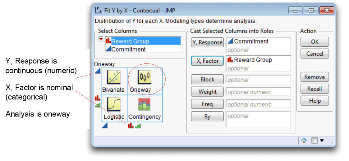
![]() When the launch dialog appears, select Reward Group, and then click X, Factor.
When the launch dialog appears, select Reward Group, and then click X, Factor.
![]() Select Commitment, and then click Y, Response.
Select Commitment, and then click Y, Response.
Your completed dialog should look like the one in Figure 8.3. Note that the modeling type of the variables, shown by the icon to the left of the variable name, determines the type of analysis. The legend in the lower-left corner of the dialog describes the type of analysis appropriate for all combinations of Y and X variable modeling types. It is important to note that you don’t have to specifically request a one-way ANOVA—the platform is constructed to perform the correct analysis based on modeling types. The type of analysis shows at the top-left of the legend and in the legend cell that represents the modeling types of the two variables.
Figure 8.3: Fit Y by X Dialog for One-Way ANOVA
Results from the JMP Analysis
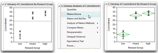
![]() Click OK to see the initial scatterplot shown on the left in Figure 8.4.
Click OK to see the initial scatterplot shown on the left in Figure 8.4.
You suspect from looking at the scatterplot that the “high” and “mixed” groups are the same and that both of these groups are significantly different from the “low” group.
![]() Choose Means/Anova from the menu on the Oneway Analysis title bar to see the scatter plot on the right and the Oneway Anova analysis report (shown and explained later).
Choose Means/Anova from the menu on the Oneway Analysis title bar to see the scatter plot on the right and the Oneway Anova analysis report (shown and explained later).
The F test in the analysis is significant (p < 0.0001), and the means diamonds visually support the conjecture about group differences. The diamonds for the “high” and “mixed” groups do not separate sufficiently to indicate a difference, but both are visibly above the “low” group.
Figure 8.4: Graphical Results of One-Way ANOVA
![]() To confirm the visual group comparison, select Compare Means from the menu on the title bar, and select All Pairs, Tukey HSD from its submenu, as shown here. Figure 8.5 shows the ANOVA results and the comparison of group means.
To confirm the visual group comparison, select Compare Means from the menu on the title bar, and select All Pairs, Tukey HSD from its submenu, as shown here. Figure 8.5 shows the ANOVA results and the comparison of group means.
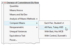
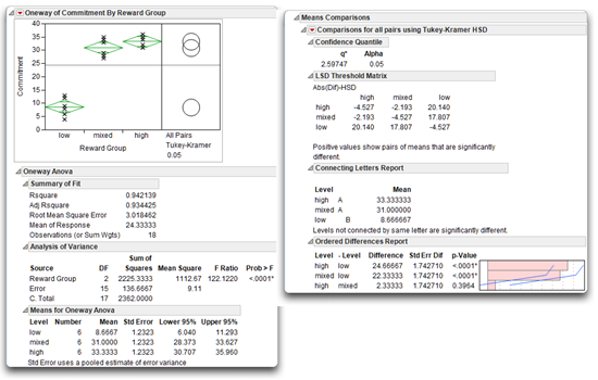
Figure 8.5: Results of ANOVA with Means Comparisons
Steps to Interpret the Results
Step 1: Make sure that everything looks reasonable. Note the analysis title and the scatterplot to verify you have completed the intended analysis. The title bar should state “Oneway Analysis of Commitment (response). By Reward Group (predictor).” The name of the response appears on the y-axis and the predictor on the x-axis.
The Summary of Fit table shows N = 18, which is the number of observations used in the analysis. This N is also the total number of participants for whom you have a complete set of data. A complete set of data means the number of participants for whom you have scores on both the predictor variable and the response variable. The degrees of freedom is 2 for Reward Group in the Analysis of Variance table, which is the number of groups (3) minus 1. The total corrected degrees of freedom (C. Total) is always equal to N – 1 = 18 – 1 = 17. If any of this basic data does not look correct, you might have made an error in entering or modifying the data.
The means for the three experimental groups are listed in the Means for Oneway Anova table. Notice they range from 8.67 through 33.33. Remember that your participants used a scale that could range from 4 through 36, so these group means appear reasonable. If these means had taken on values outside this range, there was a probable error when entering the data.
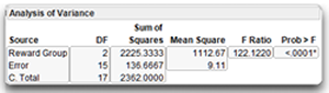
Step 2: Review the appropriate F statistic and its associated p-value. Once you verify there are no obvious errors, continue to review the results.
Look at the F statistic in the Analysis of Variance table, shown here, to see if you can reject the null hypothesis. You can state the null hypothesis for the present study as follows:
“In the population, there is no difference between the high-reward group, the mixed-reward group, and the low-reward group with respect to mean commitment scores.”
Symbolically, you can represent the null hypothesis this way:
H0: µ1 = µ 2 = µ 3
where µ 1 is the mean commitment score for the population of people in the low-reward condition, µ 2 is the mean commitment score for the population of people in the mixed-reward condition, and µ 3 is the mean commitment score for the population of people in the high-reward condition.
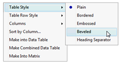
Note: The Analysis of Variance table shown previously uses the Beveled option. To change the appearance of any results table, right-click on the table, and choose the option you want.
The line in the Analysis of Variance table denoted by the predictor variable name, Reward Group, shows the statistical information appropriate for the null hypothesis, µ1 = µ 2 = µ 3.
- The heading called Source stands for source of variation. The first item under Source is the predictor (or model) variable, Reward Group. Its degrees of freedom, DF, is 2. The degrees of freedom associated with a predictor are equal to k – 1, where k represents the number of experimental groups.
- The Sum of Squares (SS for short) associated with the predictor variable, Reward Group, is 2225.33. It is found by subtracting the Error SS from the total SS found in the Analysis of Variance table. Compare the predictor (Reward Group) SS to the total SS (C. Total) to see how much of the variation in the Commitment data is accounted for by the predictor variable.
Note: The ratio of the predictor SS to the corrected SS gives the R2 (Rsquare) statistic found in the Summary of Fit table. This is the proportion of variation explained by the predictor variable, Reward Group. In this example the R2 is 2225.33 / 2362.00 = .942. This means that 94.2% of the total variation in the Commitment data is accounted for by the between groups variation of Reward Group variable. This is a very high value of R2, much higher than you are likely to obtain in an actual investigation (remember that the present data are fictitious).
- The Mean Square for Reward Group, also called the mean square between groups, is the sum of squares (2225.33) divided by its associated degrees of freedom (2), giving 1112.67. This quantity is used to compute the F ratio needed to test the null hypothesis.
- The F statistic (F Ratio) to test the null hypothesis is 122.12, which is very large. It is computed as the ratio of the model (Reward Group) mean square to the Error mean square, 1112.6667 / 9.1111 = 122.12.
- The probability (Pr > F) associated with the F ratio is less than 0.0001. This is the probability of obtaining (by chance alone) an F statistic as large or larger than the one in this analysis if the null hypothesis were true. When a p-value is less than 0.05, you often choose to reject the null hypothesis. In this example you reject the null hypothesis of no population differences. In other words, you conclude that there is a significant effect for the type of rewards independent variable.
Because the F statistic is significant, you reject the null hypothesis of no differences in population means. Instead, you tentatively conclude that at least one of the population group means is different from at least one of the other population group means. However, because there are three experimental conditions, you now have a new problem: which of these groups is significantly different from the others?
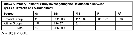
Step 3: Prepare your own version of the ANOVA summary table. Before moving on to interpret the sample means for the three experimental groups, you should prepare your own version of the ANOVA summary table (see Table 8.1). All of the information you need is presented in the Analysis of Variance table shown in Figure 8.5 except for the R2 value. However, the R2 value is shown in the Summary of Fit table. The reward group information is copied directly from the Analysis of Variance table. The within-groups information deals with the error variance in your sample and is denoted Error in the Analysis of Variance table. The total is denoted C. Total in the JMP results. You do not need to include the p-value in the table. Instead, mark the significant F value with an asterisk (*). At the bottom of the table place a note that indicates the level of significance.
You can use the R2 value in the Summary of Fit table or easily calculate R2 by hand as
Reward Group SS / C. Total SS = 2225.33 / 2362 = 0.9421
The R2 of 0.94 indicates that 94% of the variance in commitment is accounted for by the type of rewards independent variable. This is a very high value of R2, much higher than you are likely to obtain in an actual investigation.
Table 8.1: An Alternative ANOVA Summary Table
Step 4: Review the sample means and multiple comparison tests. When you request any means comparison test, means comparison circles for that test appear next to the scatterplot, as shown here and in Figure 8.5. The horizontal radius of a circle aligns to its respective group mean on the scatterplot. You can quickly compare each pair of group means visually by examining how the circles intersect.
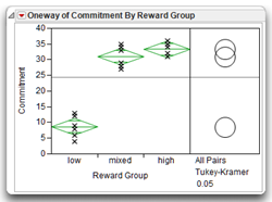
- Means comparison circles that do not overlap or overlap only slightly represent groups that significantly different.
- Circles with significant overlapping (such as those for the “mixed” and “high” groups) represent group means that are not different.
See Basic Analysis and Graphing (2012), which is available from the Help menu, and Sall (1992) for a detailed discussion of means comparison circles.
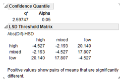
Step 5: Review the Means Comparisons report. The results of the Means Comparisons test were shown previously in Figure 8.5. At the top of the Means Comparisons report you see an alpha level of 0.05. This alpha level means that if any of the groups are significantly different from the others, they are different with a significance level of p < 0.05. The results give the following information:
- To the left of the alpha at the top of the report, you see a q* value of 2.59747. The q statistic is the quantile used to scale the Least Significant Difference (LSD) values. This value plays the same role in the computations as the t quantile in t-tests that compare group means. Using a t-test to compare more than two group means gives significance values that are too liberal. The q value is constructed to give more accurate probabilities. If the Tukey-Kramer test finds significant differences between any pair of means, they are said to be “Honestly Significant Differences.” Thus, this test is called the Tukey-Kramer HSD test.
Next you see a table of the actual absolute difference in the means minus the LSD (shown here). The Least Significant Difference (LSD) is the difference that woul be significant. Pairs with a positive value are significantly different.
- The Tukey letter grouping shows the mean scores for the three groups on the response variable (the Commitment variable in this study) and whether or not these group means are different. You can see that the high-reward group has a mean commitment score of 33.3, the mixed-reward group has a mean score of 31.0, and the low-reward group had a mean score of 8.7. The letter A identifies the high-reward group and the letter B identifies the low-reward group. You conclude these two groups have significantly different mean Commitment scores.
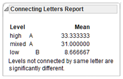
Similarly, different letters also identify the mixed-reward and low-reward groups, so their means are significantly different. However, the letter A identifies both the high-reward and mixed-reward groups. Therefore, the means of these two groups are not significantly different.
- The difference between each pair of means shows at the bottom of this report, with lower and upper confidence limits for each pair. The bar chart of the differences, ordered from high to low, gives another quick visual comparison.
Examining the means comparison circles for Tukey’s HSD test and the Means Comparisons report, you can conclude there was no significant difference in the mean response of the high-reward group and the mixed-reward group. However, there is a significant difference between the low-reward group means and the other two group means.
Note: Remember that you should review the results of a multiple comparison procedure only if the F value from the preceding Analysis of Variance table is statistically significant.
Summarize the Results of the Analysis
When performing a one-factor ANOVA, you can use the following format to summarize the results of your analysis:
A. Statement of the problem
B. Nature of the variables
C. Statistical test
D. Null hypothesis (Ho)
E. Alternative hypothesis (H1)
F. Obtained statistic (F)
G. Obtained probability (p) value
H. Conclusion regarding the null hypothesis
I. Magnitude of the treatment effect (R2)
J. ANOVA summary table
K. Figure representing the results
Here is an example summary for the one-way analysis of variance.
A. Statement of the problem
The purpose of this study was to determine if there was a difference between people in a high-reward relationship, a mixed-reward relationship, or a low-reward relationship, with respect to their commitment to the relationship.
B. Nature of the variables
This analysis involved two variables. The predictor variable was types of reward, which was measured on a nominal scale and could assume one of three values: a low-reward condition, a mixed-reward condition, and a high-reward condition. The numeric continuous response variable represented subjects’ commitment.
C. Statistical test
One-way anova, between-subjects design.
D. Null hypothesis (H0)
µ1 = µ 2 = µ 3; in the population, there is no difference between subjects in a high-reward relationship, subjects in a mixed-reward relationship, and subjects in a low-reward relationship with respect to their mean commitment scores.
E. Alternative hypothesis (H1)
In the population, there is a difference between at least two of the following three groups with respect to their mean commitment scores: subjects in a high-reward relationship, subjects in a mixed-reward relationship, and subjects in a low-reward relationship.
F. Obtained statistic
F(2,15) = 122.12.
G. Obtained probability (p) value
p < 0.0001.
H. Conclusion regarding the null hypothesis
Reject the null hypothesis.
I. Magnitude of the treatment effect
R2 = 0.94 (large treatment effect)
J. ANOVA Summary table
See Table 8.1.
K. Figure representing the results
Like the chart shown here, generated by the Chart command in the Graph menu.
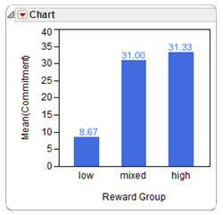
To produce the bar chart shown here, do the following:
![]() Choose the Chart command from the Graph menu.
Choose the Chart command from the Graph menu.
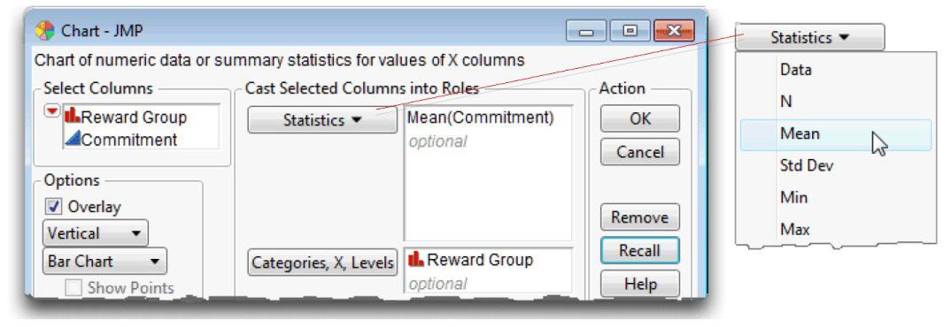
![]() On the launch dialog, select Reward Group as X. Select Commitment and choose Mean from the Statistics menu in the dialog, as shown in Figure 8.6, and click OK to see the bar chart.
On the launch dialog, select Reward Group as X. Select Commitment and choose Mean from the Statistics menu in the dialog, as shown in Figure 8.6, and click OK to see the bar chart.
![]() Use the annotate tool (
Use the annotate tool (![]() ) found on the Tools menu or on the tool bar to label the bars with their respective mean values given in the analysis results. Alternatively, use options in the red triangle menu on the Chart title bar to add labels to the bars.
) found on the Tools menu or on the tool bar to label the bars with their respective mean values given in the analysis results. Alternatively, use options in the red triangle menu on the Chart title bar to add labels to the bars.
Figure 8.6: Completed Chart Launch Dialog to Chart Group Means
Formal Description of Results
You could use the following approach to summarize this analysis for a paper in a professional journal:
Results were analyzed using a one-way ANOVA, between-subjects design. This analysis revealed a significant effect for type of rewards, F(2,15) = 122.12; p < 0.001. The sample means are displayed in Figure 8.5. Tukey’s HSD test showed that subjects in the high-reward and mixed-reward conditions scored significantly different on commitment than did subjects in the low-reward condition (p < 0.05). There were no significant differences between subjects in the high-reward condition and subjects in the mixed-reward condition.
Example with Nonsignificant Differences between Experimental Conditions
In this section you repeat the preceding analysis on a data table designed to provide nonsignificant results. This will help you learn how to interpret and summarize results when there are no significant differences between group differences. The data table for this example is mixed reward nodiff.jmp, which is shown here.
Use the same steps described for the previous example to analyze the data.
![]() Choose Fit Y by X from the Analyze menu.
Choose Fit Y by X from the Analyze menu.
![]() When the launch dialog appears, select Reward Group and click X, Factor.
When the launch dialog appears, select Reward Group and click X, Factor.
![]() Select Commitment and click Y, Response.
Select Commitment and click Y, Response.
![]() Click OK in the launch dialog to see the results in Figure 8.7.
Click OK in the launch dialog to see the results in Figure 8.7.
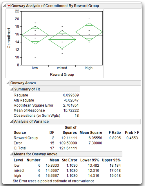
Again, you are most interested in the Analysis of Variance table. The F statistic (F Ratio) for this analysis is 0.8295, with associated probability (Prob > F) of 0.4553. Because this p-value is greater than .05, you fail to reject the null hypothesis and conclude that the types of reward independent variable did not have a significant effect on rated commitment.
The Means for Oneway Anova table shows the mean scores on Commitment for the three groups. You can see that there is little difference between these means as all three groups display an average score on Commitment between 14 and 17. You can use the scatterplot with means diamonds to graphically illustrate results, or use the mean values from the analysis to prepare a bar chart like the one describe in the previous section.
Figure 8.7: Results of ANOVA for Example with No Differences
Summarizing the Results of the Analysis with Nonsignificant Results
This section summarizes the present results according to the statistical interpretation format presented earlier. Because the same hypothesis is being tested, items A through E are completed in the same way as before. Therefore, only items F through J are presented here. Refer to the results shown in
Figure 8.7.
F. Obtained statistic
F(2,15) = 0.8395
G. Obtained probability (p) value
p = 0.4553 (not significant)
H. Conclusion regarding the null hypothesis
Fail to reject the null hypothesis.
I. Magnitude of treatments effect
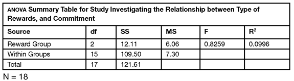
R2 = Reward Group SS / C. Total SS = 12.11 / 121.61 = 0.0996
J. ANOVA Summary table
See Table 8.2.
Table 8.2: An Alternative ANOVA Summary Table
K. Figure representing results
See means diamonds plot in Figure 8.7, or prepare bar chart as shown for previous example.
Formal Description of Results
You could summarize the results from the present analysis in the following way for a published paper:
Results were analyzed using a one-way ANOVA, between-subjects design. This analysis failed to reveal a significant effect for type of rewards, F(2,15) = 0.83, not significant with negligible treatment effect of R2 = 0.10. The sample means are displayed in Figure 8.7, which shows that the three experimental groups demonstrated similar commitment scores.
Understanding the Meaning of the F Statistic
An earlier section mentioned that you obtain significant results in an analysis of variance when the F statistic produced in the Analysis of variance assumes a relatively large value. This section explains why this is so.
The meaning of the F statistic might be easier to understand if you think about it in terms of what results would be expected if the null hypothesis were true. If there really were no differences between groups with respect to their means, you expect to obtain an F statistic close to 1.00. In the previous analysis, the obtained F value was much larger than 1.00 and, although it is possible to obtain an F of 122.12 when the population means are equal, it is extremely unlikely. In fact, the calculated probability, the p-value, in the analysis was less than or equal to 0.0001 (less than 1 in 10,000)). Therefore, you rejected the null hypothesis of no population differences.
But why do you expect an F value of 1.00 when the population means are equal? And why do you expect an F value greater than 1.00 when the population means are not equal? To understand this, you need to understand how the F statistic is calculated. The formula for the F statistic is as follows:
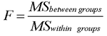
- The numerator in this ratio is MSbetween groups, which represents the mean square between groups. This between-subjects variability is influenced by two sources of variation—error variability and variability due to the differences in the population means.
- The denominator in this ratio is MSwithin groups, which represents the mean square within groups. The within-groups variability is the sum of the variability measures that occur within each single treatment group. This is a measure of variability that is influenced by only one source of variation—error variability. For this reason, the MSwithin groups is often referred to as the MSerror.
Now you can see why the F statistic should be larger than 1.00 when there are differences in population means (when the null hypothesis is incorrect). Consider writing the formula for the F statistic as follows:
![]() If the means are different, the predictor variable (types of reward) has an effect on commitment. Therefore, the numerator of the F ratio contains two sources of variation—both error variability plus variability due to the differences in the population means. However, the denominator (MSwithin groups) is influenced by only one source of variance—error variability. Note that both the numerator and the denominator are influenced by error variability, but the numerator is affected by an additional source of variance, so the numerator should be larger than the denominator. Whenever the numerator is larger than the denominator in a ratio, the resulting quotient is greater than 1.00. In other words, you expect to see an F value greater than 1.00 when there are differences between means. It follows that you reject the null hypothesis of no population differences when you obtain a sufficiently large F statistic.
If the means are different, the predictor variable (types of reward) has an effect on commitment. Therefore, the numerator of the F ratio contains two sources of variation—both error variability plus variability due to the differences in the population means. However, the denominator (MSwithin groups) is influenced by only one source of variance—error variability. Note that both the numerator and the denominator are influenced by error variability, but the numerator is affected by an additional source of variance, so the numerator should be larger than the denominator. Whenever the numerator is larger than the denominator in a ratio, the resulting quotient is greater than 1.00. In other words, you expect to see an F value greater than 1.00 when there are differences between means. It follows that you reject the null hypothesis of no population differences when you obtain a sufficiently large F statistic.
In the same way, you can also see why the F statistic should be approximately equal to 1.00 when there are no differences in means values (when the null hypothesis is correct). Under these circumstances, the predictor variable (level of rewards) has no effect on commitment. Therefore, the MSbetween groups is not influenced by variability due to differences between the means. Instead, it is influenced only by error variability. So the formula for the F statistic reduces to:
![]()
The number in the numerator in this formula is fairly close to the number in the denominator. Whenever a numerator in a ratio is approximately equal to the denominator in that ratio, the resulting quotient is close to 1.00. Hence, when a predictor variable has no effect on the response variable, you expect an F statistic close to 1.00.
Summary
The one-way analysis of variance is one of the most flexible and widely used procedures in the social sciences. It allows you to test for significant differences between groups, and its applicability is not limited to studies with just two groups (as the t-test is limited). However, an even more flexible procedure is the factorial analysis of variance. Factorial ANOVA allows you to analyze data from studies in which more than one independent variable is manipulated. Not only does this allow you to test more than one hypothesis in a single study, but it also allows you to investigate an entirely different type of effect called an “interaction.” Factorial analysis of variance is introduced in the following chapter.
Appendix: Assumptions Underlying One-Way ANOVA with One Between-Subjects Factor
Modeling type
The response variable should be assessed on an interval-level or ratiolevel of measurement. The predictor variable should be a nominal-level variable (a categorical variable) that includes two or more categories.
Independent observations
A given observation should not be dependent on any other observation in any group (for a more detailed explanation of this assumption, see Chapter 7).
Random sampling
Scores on the response variable should represent a random sample drawn from the populations of interest.
Normal distributions
Each group should be drawn from a normally distributed population. If each group has 30 or more subjects, the test is robust against moderate departures from normality.
Homogeneity of variance
The populations represented by the various groups should have equal variances on the response. If the number of subjects in the largest group is no more than 1.5 times greater than the number of subjects in the smallest group, the test is robust against violations of the homogeneity assumption (Stevens, 1986).
References
Hatcher, L. 2003. Step-by-Step Basic Statistics Using SAS. Cary, NC: SAS Institute Inc.
Sall, J. 1992. “Graphical Comparison of Means.” American Statistical Association Statistical Computing and Statistical Graphics Newsletter, 3, 27–32.
SAS Institute Inc. 2012. Basic Analysis and Graphing. Cary, NC: SAS Institute Inc.
Stevens, J. 1986. Applied Multivariate Statistics for the Social Sciences. Hillsdale, NJ: Lawrence Erlbaum Associates.