14

Principal Component Analysis

Overview

This chapter provides an introduction to principal component analysis, which is a variable-reduction procedure similar to factor analysis. It provides guidelines regarding the necessary sample size and number of items per component. It shows how to determine the number of components to retain, interpret the rotated solution, create factor scores, and summarize the results. Fictitious data are analyzed to illustrate these procedures. This chapter deals only with the creation of orthogonal (uncorrelated) components.

Overview

Introduction to Principal Component Analysis

A Variable Reduction Procedure

An Illustration of Variable Redundancy

Number of Components Extracted

What Is a Principal Component?

Principal Component Analysis Is Not Factor Analysis

The Prosocial Orientation Inventory

Preparing a Multiple-Item Instrument

Number of Items per Component

Minimally Adequate Sample Size

Using JMP for Principal Components Analysis

Conduct the Principal Component Analysis

Step 1: Extract the Principal Components

Step 2: Determine the Number of Meaningful Components

Step 3: Rotate to a Final Solution

Step 4: Interpret the Rotated Solution

Step 5: Create Factor Scores or Factor-Based Scores

Step 6: Summarize Results in a Table

Step 7: Prepare a Formal Description of Results for a Paper

Summary

Appendix: Assumptions Underlying Principal Component Analysis

References

Introduction to Principal Component Analysis

Principal component analysis is an appropriate procedure when you have measures on a number of observed variables and want to develop a smaller number of variables (called principal components) that account for most of the variance in the observed variables. The principal components can then be used as predictors or response variables in subsequent analyses. Additionally, principal components representation is important in visualizing multivariate data by reducing it to dimensionalities that are graphable.

A Variable Reduction Procedure

Principal component analysis is a variable reduction procedure. It is useful when you obtain data for a number of variables (possibly a large number of variables) and believe that there is redundancy among those variables. In this case, redundancy means there is correlation among subsets of variables. Because of this redundancy, you believe it should be possible to reduce the observed variables into a smaller number of principal components that will account for most of the variance in the observed variables. Further, principal components representation is important in visualizing multivariate data by reducing it to dimensionalities that are graphable.

Because principal component analysis is a variable reduction procedure, it is similar to exploratory factor analysis. In fact, the steps followed in a principal component analysis are identical to those followed when conducting an exploratory factor analysis. However, there are significant conceptual differences between the two procedures. It is important not to claim you are performing factor analysis when you are actually performing principal component analysis. The “Principal Component Analysis Is Not Factor Analysis” section in this chapter describes the differences between these two procedures.

An Illustration of Variable Redundancy

The following fictitious research example illustrates the concept of variable redundancy. Imagine that you develop a seven-item questionnaire like the one shown in Table 14.1, which is designed to measure job satisfaction. You administer this questionnaire to 200 employees and use their responses to the seven items as seven separate variables in subsequent analyses.

There are a number of problems with conducting the study in this manner. One of the more important problems involves the concept of redundancy, which was mentioned previously. Examine the content of the seven items in the questionnaire closely. Notice that items 1 to 4 deal with the employees’ satisfaction with their supervisors. In this way, items 1 to 4 are somewhat redundant. Similarly, notice that items 5 to 7 appear to deal with the employees’ satisfaction with their pay.

Table 14.1: Questionnaire to Measure Job Satisfaction

Empirical findings might further support the notion that there is redundancy among items. Assume that you administer the questionnaire to 200 employees and compute all possible correlations between responses to the seven items. Table 14.2 shows correlations from this fictitious data.

When correlations among several variables are computed, they are typically summarized in the form of a correlation matrix such as the one presented in Table 14.2. The rows and columns in Table 14.2 correspond to the seven variables included in the analysis. Row 1 and column 1 represent variable 1, row 2 and column 2 represents variable 2, and so forth. The correlation for a pair of variables appears where a given row and column intersect. For example, where the row for variable 2 intersects with the column for variable 1, you find a correlation of 0.75. This means that the correlation between variable 1 and variable 2 is 0.75.

Table 14.2: Correlations among Seven Job Satisfaction Items for 200 Responses

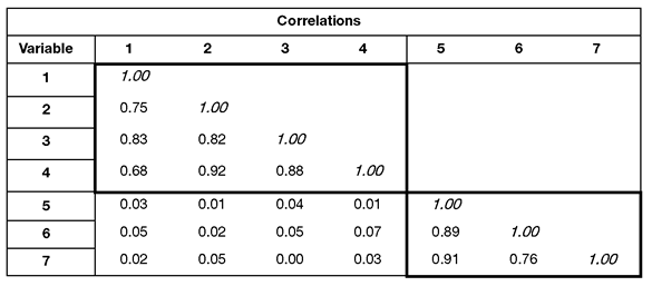
The correlations in Table 14.2 show that the seven items seem to form two distinct groups. First, notice that items 1 to 4 show relatively strong correlations with one another. This could be because items 1 to 4 measure the same construct. Similarly, items 5 to 7 correlate strongly with one another, which is a possible indication that they also measure the same construct. Also notice that items 1 to 4 show very weak correlations with items 5 to 7. This is what you expect to see if items 1 to 4 and items 5 to 7 are measuring two different constructs.

Given this apparent redundancy, it is likely that the seven items of the questionnaire do not measure seven different constructs. More likely, items 1 to 4 measure a single construct that could reasonably be labeled “satisfaction with supervision” whereas items 5 to 7 measure a different construct that could be labeled “satisfaction with pay.”

If the responses to the seven items actually displayed the redundancy suggested by the pattern of correlations in Table 14.2, it would be advantageous to reduce the number of variables so that items 1 to 4 collapse into a single new variable and items 5 to 7 collapse into a second new variable. You could then use these two new variables (instead of the seven original variables) as predictor variables in a multiple regression or any other type of analysis.

Number of Components Extracted

The number of components extracted (created) in a principal component analysis is equal to the number of observed variables being analyzed. This means that an analysis of the seven-item questionnaire can result in seven components.

However, in most analyses only the first few components account for meaningful amounts of variance so only these first few components are interpreted and used in a subsequent analyses such as a multiple regression. For example, in the analysis of the seven-item job satisfaction questionnaire, it is likely that only the first two components will reflect the redundancy in the data and account for a meaningful amount of variance. Therefore, only these components would be retained for use in subsequent analysis. You assume that the remaining five components account for only trivial amounts of variance. These latter components are not retained, interpreted, or further analyzed.

Principal component analysis is a mathematical way of collapsing variables. It allows you to reduce a set of observed variables into a set of variables called principal components. A subset of these principal components accounts for a significant portion of the variability in the data and can then be used in subsequent analyses.

What Is a Principal Component?

Technically, a principal component can be defined as a linear combination of optimally weighted observed variables. In order to understand the meaning of this definition, it is necessary to first describe how participant scores on a principal component are computed.

How Principal Components Are Computed

In the course of performing a principal component analysis, it is possible to calculate a score for each participant for a given principal component. Participants’ actual scores on the seven questionnaire items are optimally weighted and then summed to compute their scores for a given component.

The general form for the formula to compute scores on the first component extracted in a principal component analysis follows:

C1 = b11(X1) + b12(X2) + ... b1p(Xp)

where

C1 = the participant’s score on principal component 1 (the first component extracted, sometimes denoted PC1)

B1p = the regression coefficient (or weight) for observed variable p, as used in creating principal component 1

Xp = the participant’s score on observed variable p

For example, you can determine each participant’s score on the first principal component by using the following fictitious formula:

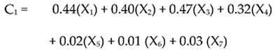
In this case, the observed variables (the X variables) are responses to the seven job satisfaction questions: X1 represents question 1, X2 represents question 2, and so forth. Notice that different regression coefficients are assigned to the different questions to scores on C1 (principal component 1). Questions 1 to 4 have larger regression weights that range from 0.32 to 0.44, whereas questions 5 to 7 have smaller weights ranging from 0 .01 to 0.03.

A different equation with different weights computes scores on component 2 (PC2). Below is a fictitious illustration of this formula:

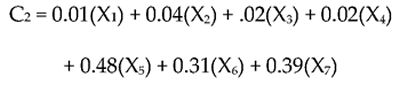
The preceding equation shows that, in creating scores on the second component, items 5 to 7 have higher weights and items 1 to 4 have lower weights.

Notice how the weighting for component 1 and component 2 reflect the questionnaire design and variable redundancy shown in the correlation table (Table 14.2).

• PC1 accounts for the most of the variability in the “satisfaction with supervision” items. Satisfaction with supervision is assessed by questions 1 to 4. You expect that items 1 to 4 have more weight in computing participant scores on this component and items 5 to 7 have less. Component 1 will be strongly correlated with items 1 to 4.
• PC32 accounts for much of the variability in the “satisfaction with pay” items. You expect that items 5 to 7 have more weight in computing participant scores on this component and items 1 to 4 have less. Component 2 will be strongly correlated with items 5 to 7.

Optimal Weights for Principal Components

At this point, it is reasonable to wonder how the regression weights from the preceding equations are determined. The JMP Principal Components platform generates these weights by computing eigenvalues. An eigenvalue is the amount of variance captured by a given component or factor. The eigenvalues are optimal weights in that, for a given set of data, no other weights produce a set of components that are more effective in accounting for variance among observed variables. The weights satisfy a principle of least squares similar (but not identical) to the principle of least squares used in multiple regression (see Chapter 13, “Multiple Regression”). Later, this chapter shows how the Principal Components platform in JMP can be used to extract (create) principal components.

It is now possible to understand the definition provided at the beginning of this section more fully. A principal component is defined as a linear combination of optimally weighted observed variables. The term linear combination means that the component score is created by adding together weighted scores on the observed variables being analyzed. Optimally weighted means that the observed variables are weighted in such a way that the resulting components account for a maximum amount of observed variance in the data. No other set of weights can account for more variation.

Characteristics of Principal Components

The first principal component extracted in a principal component analysis accounts for a maximal amount of total variance in the observed variables. Under typical conditions, this means that the first component is correlated with at least some of the observed variables. In fact, it is often correlated with many of the variables.

The second principal component extracted has two important characteristics.

• PC2 accounts for a maximal amount of variance in the data not accounted for by the PC1. Under typical conditions, this means that PC2 is correlated with some of the observed variables that did not display strong correlations with first component.
• The second characteristic of PC2 is that it is uncorrelated with the PC1. If you compute the correlation between PC1 and PC2, that correlation is zero.

The remaining components extracted in the analysis display these same two characteristics—each component accounts for a maximal amount of variance in the observed variables that was not accounted for by the preceding components and is uncorrelated with all of the preceding components. A principal component analysis proceeds in this manner with each new component accounting for progressively smaller amounts of variance. This is why only the first few components are retained and interpreted. When the analysis is complete, the resulting components display varying degrees of correlation with the observed variables, but are completely uncorrelated with one another.

What Is the Total Variance in the Data?

To understand the meaning of total variance as it is used in a principal component analysis, remember that the observed variables are standardized in the course of the analysis. This means that each variable is transformed so that it has a mean of zero and a standard deviation of one (and hence a variance of one). The total variance in the data is the sum of the variances of these observed variables. Because they have been standardized to have a standard deviation of one, each observed variable contributes one unit of variance to the total variance in the data. Therefore, the total variance in a principal component analysis always equals to the number of observed variables analyzed—if seven variables are analyzed, then the total variance is seven.

Note: The total number of components extracted in the principal component analysis partition the total variance. That is, the sum of the variance accounted for by all principal components is the total variation in the data.

Principal Component Analysis Is Not Factor Analysis

Principal component analysis is often confused with factor analysis. There are many important similarities between the two procedures. Both methods attempt to identify groups of observed variables. Both procedures can be performed with the Multivariate platform and often provide similar results.

The purpose of both common factor analysis and principal component analysis is to reduce the original variables to fewer composite variables, which are called factors or principal components. However, these two analyses have different underlying assumptions about the variance in the original variables, and the obtained composite variables serve different purposes.

In principal component analysis, the objective is to account for the maximum portion of the variance present in the original set of variables with a minimum number of composite variables (principal components). The assumption is that the error (unique) variance represents a small portion of the total variance in the original set of variables. Principal components analysis does not make a distinction between common (shared) and unique parts of the variation in a variable.

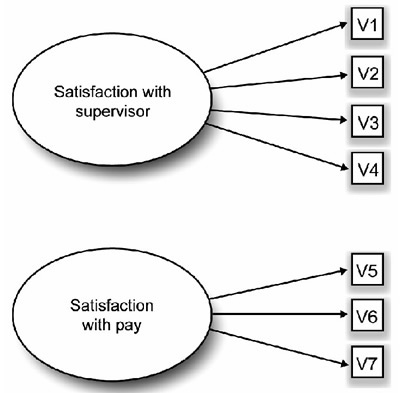
In factor analysis, a small number of factors are extracted to account for the correlations among the observed variables—to identify the latent dimensions that explain why the variables are correlated with each other. The observed variables are only indicators of the latent constructs to be measured. The assumption is that the error (unique) variance represents a significant portion of the total variance and that the variation in the observed variables is due to the presence of one or more latent variables (factors) that exert causal influence on these observed variables. An example of such a causal structure is presented in Figure 14.1.

The ovals in Figure 14.1 represent the latent (unmeasured) factors of “satisfaction with supervision” and “satisfaction with pay.” These factors are latent in the sense that they are assumed to actually exist in the employees’ belief systems but are difficult to measure directly. However, they do exert an influence on the employees’ responses to the seven items in the job satisfaction questionnaire in Table 14.1. These seven items are represented as the squares labeled V1 to V7 in the figure. It can be seen that the “supervisor” factor exerts influence on items V1 to V4 and the “pay” factor exerts influence on items V5 to V7.

Researchers use factor analysis when they believe latent factors exist that exert causal influence on the observed variables they are studying. Exploratory factor analysis helps the researcher identify the number and nature of these latent factors.

In contrast, principal component analysis makes no assumption about an underlying causal structure. Principal component analysis is a variable reduction procedure that can result in a relatively small number of components that account for most of the variance in a set of observed variables.

Figure 14.1: Example of the Underlying Causal Structure Assumed in Factor Analysis

In summary,

• Factor analysis groups variables under the assumption that the groups represent latent constructs. Factor analysis attempts to identify these constructs but is not expected to extract all variability from the data. A factor analysis only uses the variability in an item that it has in common with the other items (its communality).
• Principal component analysis produces a set of orthogonal (uncorrelated) linear combinations of the variables. The first principal component accounts for the most possible variance in the data. The second component accounts for the most variance not accounted for by the first component, and so on until all variability is accounted for. The first few components account for most of the total variation in the data and can be used for subsequent analysis.

Both factor analysis and principal component analysis have important roles to play in social science research, but their conceptual foundations are quite distinct. In most cases, these two methods yield similar results. However, principal components analysis is often preferred as a method for data reduction, while principal factors analysis is often preferred when the goal of the analysis is to detect structure.

The Prosocial Orientation Inventory

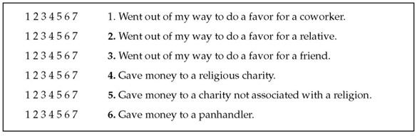
Assume that you have developed an instrument called the Prosocial Orientation Inventory (POI) that assesses the extent to which a person has engaged in types of “helping behavior” over the preceding six-month period. The instrument contains six items and is presented in Table 14.3.

When this instrument was first developed, you intended to administer it to a sample of participants and use their responses to the six items as separate predictor variables in a multiple regression equation. As previously stated, you learned that this is a questionable practice and decide instead to perform a principal component analysis on responses to the six items to see if a smaller number of components can successfully account for most of the variance in the data. If this is the case, you will use the resulting components as the predictor variables in your regression analyses.

At this point, it may be instructive to review the content of the six items in Table 14.3 that constitute the prosocial orientation inventory (POI) to make an informed guess as to what you are likely to observe from the principal component analysis. Imagine that, when you first constructed the instrument, you assumed that the six items were assessing six different types of prosocial behavior. However, inspection of items 1 to 3 shows that these three items appear to share something in common—they deal with “going out of one’s way to do a favor for someone else.” It would not be surprising to learn that these three items are highly correlated and group together in the principal component analysis to be performed. In the same way, a review of items 4 to 6 shows that all of these items involve “giving money to those in need.” These three items might also be correlated and form the basis of a second principle component.

Table 14.3: The Prosocial Orientation Inventory (POI)

In summary, the nature of the items suggests that it may be possible to account for the variance in the POI with just two components that will be a “helping others” component and a “financial giving” component. At this point, this is only speculation. Only a formal analysis can determine the number of components measured by the POI.

Note: keep in mind that the principal component analysis does not assume the underlying constructs described above (“helping others” and “financial giving”). These speculative constructs are used here only as a possible explanation for the correlations between variables 1 to 3, and between variables 4 to 6 that ultimately result in useful principle components.

The preceding instrument is fictitious and used for purposes of illustration only. It should not be regarded as an example of a good measure of prosocial orientation. Among other problems, this questionnaire obviously deals with very few forms of helping behavior.

Preparing a Multiple-Item Instrument

The preceding section illustrates an important point about how not to prepare a multiple-item measure of a construct. Generally speaking, it is poor practice to throw together a questionnaire, administer it to a sample, and then perform a principal component analysis (or factor analysis) to determine what the questionnaire measures.

Better results are much more likely when you make a priori decisions about what you want the questionnaire to measure and then take steps to ensure that it does.

For example, in order to obtain desirable results:

• Begin with a thorough review of theory and research on prosocial behavior.
• Use that review to determine how many types of prosocial behavior probably exist.
• Write multiple questionnaire items to assess each type of prosocial behavior.

Using this approach, you could have made statements such as “there are three types of prosocial behavior—acquaintance helping, stranger helping, and financial giving.” You could then prepare a number of items to assess each of these three types and administer the questionnaire to a large sample. Then, a principal component analysis might produce three major components and a subsequent factor analysis could be used verify that three factors did emerge.

Number of Items per Component

The weight a variable such as a questionnaire item has in a principal component analysis (or a factor in a factor analysis) is its load on that component or factor. For example, if the item “Went out of my way to do a favor for a coworker” has a large weight in the first principal component, we say that the item loads on that component.

It is desirable to have at least three (and preferably more) variables loading on each retained component when the principal component analysis is complete (see Clark and Watson, 1995). Because some of the items could be dropped during the course of the analysis, it is good practice to create a questionnaire that has at least five items for each construct you want to measure. This increases the chance that at least three items per component will survive the analysis. Note that we have violated this recommendation by writing only three items for each of the two a priori components constituting the POI.

The recommendation of three items per scale offered here should be viewed as an absolute minimum and not as an optimal number of items per scale. In practice, test and attitude scale developers usually desire that their scales contain many more than just three items to measure a given construct. It is not unusual to see individual scales that include 10, 20, or more items to assess a single construct (O’Rourke and Cappeliez, 2002). The recommendation of three items per scale should therefore be viewed as a lower bound, appropriate only if practical concerns (such as total questionnaire length) prevent you from including more items. For more information on scale construction, see Spector (1992).

Minimally Adequate Sample Size

Principal component analysis is a large-sample procedure. To obtain useful results, the minimum number of participants for the analysis should be the larger of 100 participants and five times the number of variables being analyzed (Streiner, 1994).

To illustrate, assume that you want to perform an analysis on responses to a 50-item questionnaire. Remember that the number of variables to be analyzed is equal to the number of items on the questionnaire. Five times the number of items on the questionnaire equals 250. Therefore, on a 50-item questionnaire the final sample should provide usable (complete) data from at least 250 participants. Keep in mind that any participant who fails to answer even a single item does not provide usable data for the principal component analysis. To ensure that the final sample includes at least 250 usable responses, you would be wise to administer the questionnaire to perhaps 300 to 350 participants.

These rules regarding the number of participants per variable again constitute a lower bound. Some researchers argue that these rules should apply only when many variables are expected to load on each component and when variable communalities are high. Under less optimal conditions, even larger samples might be required. In factor analysis, the proportion of variance of an item that is due to common factors (shared with other items) is called communality. The principal component analysis in JMP also shows item communalities.

A communality refers to the percent of variance in an observed variable that is accounted for by the retained components (or factors). A given variable displays a large communality if it loads heavily on at least one of the study’s retained components. The concept of variable communality is more relevant in a factor analysis than in principal component analysis, but communalities are estimated in both procedures.

Using JMP for Principal Components Analysis

Principal components can be accessed from three platforms in JMP:

• Analyze > Multivariate Methods > Multivariate (red triangle option).
• Analyze > Multivariate Methods > Principal Components.
• Graph > Scatterplot 3D (a red triangle option).

All three platforms use the same routines but give different views and arrangements of the results.

This chapter begins with the Multivariate Methods > Multivariate platform to look at correlations and continues with the Multivariate Methods > Principal Components platform to extract principal components.

The Multivariate platform has options for you to choose a principal component analysis, however we use this platform to summarize the data. This first example shows correlations and a scatterplot matrix for the variables in the data table called Procial Behavior.jmp.

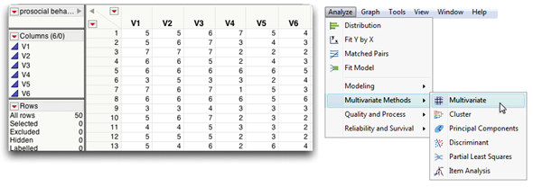
Assume that you administered the POI to 50 participants and entered their responses into a JMP table. Figure 14.2 shows the first few observations in the job satisfaction table.

Figure 14.2: The Prosocial Behavior Data Table and Multivariate Menu

The following steps show how to summarize multivariate data with tables and plots.

Open the Prosocial Behavior.jmp data table.

Choose Multivariate Methods > Multivariate from the Analyze menu.

When the Multivariate launch dialog appears, select V1-V6 in the variable list and click Y, Columns to add them to the analysis list. Click OK on the launch dialog to see the initial results in Figure 14.3.

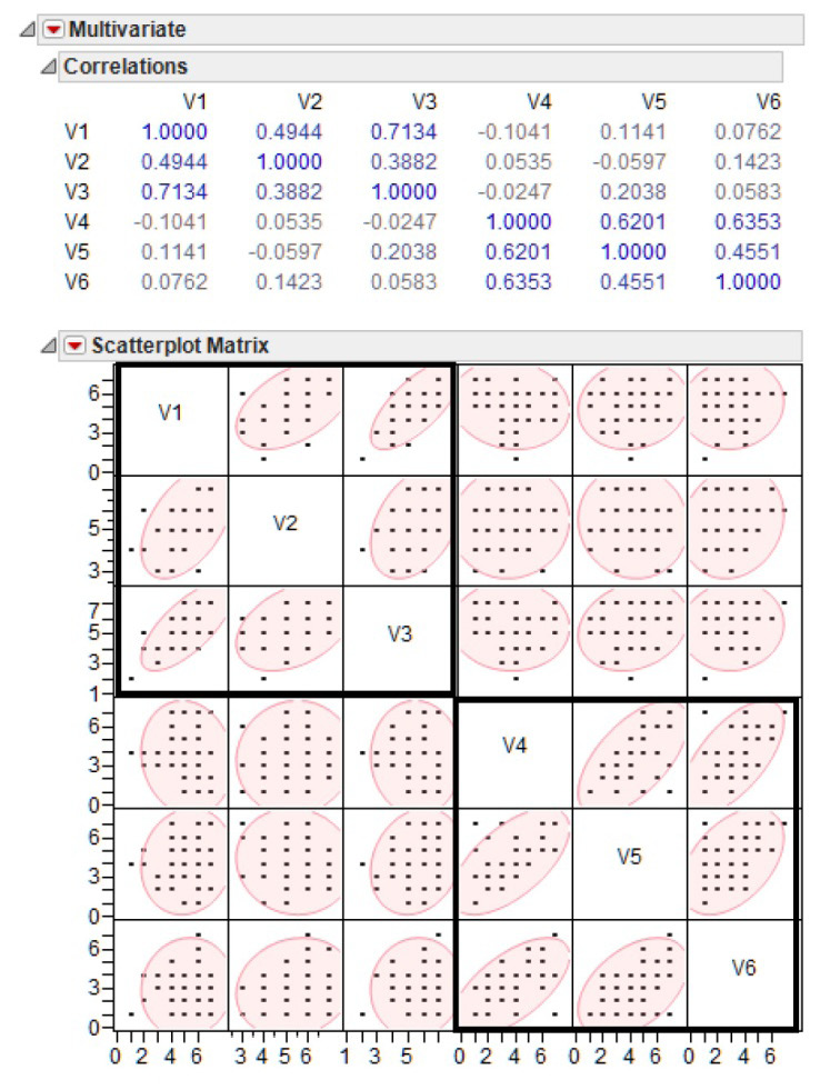
The Multivariate platform begins with a correlation matrix followed by a Scatterplot Matrix (Figure 14.3) that gives a visual representation of the correlations. Recall that the first three questionnaire items address (V1–V3) the “satisfaction with supervisor” component so you expect them to exhibit a higher correlation within each other than with the last three items, Likewise, V4–V6 address the “satisfaction with pay” component and show higher correlations with each other than with the first three items. Significantly higher correlations show bolded in the table and the Scatterplot Matrix clearly shows these correlations.

Each cell in the Scatterplot Matrix represents the correlation between the two variables listed on the horizontal and vertical axis of that cell. Options in the red triangle menu on the Multivariate title bar add features to the results. For example each cell has a 95% density ellipse overlaid on its points and the ellipse has translucent shading to better show outlying points.

When two variables are bivariate normally distributed, their ellipse encloses about 95% of the points. Variables that have higher correlations show an ellipse that is flattened and elongated on the diagonal. Variables with little correlation (correlation close to zero) show more rounded ellipse that is not diagonally oriented.

You can see in Figure 14.3 that V1–V3 show higher correlations among themselves and V4–V6 are also correlated, as expected by the design of the questionnaire.

Figure 14.3: Correlations and Scatterplot Matrix for Prosocial Data

Conduct the Principal Component Analysis

Principal component analysis is normally conducted in a sequence of steps, with somewhat subjective decisions being made at various points. Because this is an introductory treatment of the topic, it does not provide a comprehensive discussion of all of the options available to you at each step. Instead, specific recommendations are made, consistent with practices commonly followed in applied research. For a more detailed treatment of principal component analysis and factor analysis, see Kim and Mueller (1978a, 1978b), Rummel (1970), or Stevens (1986).

Step 1: Extract the Principal Components

Principal component analysis can be performed on raw data, on a correlation matrix derived from data, or on a covariance matrix derived from the data. By default, the Principal Components platform uses the correlation matrix from the data as the basis for the analysis but you have the option to specify otherwise. To extract the principal components do the following steps:

With the Prosocial Behavior data active, choose Multivariate Methods > Principal Components.

Select the 6 variables (V1–V6) and add them to the Y, Columns list, then click OK to see Figure 14.4.

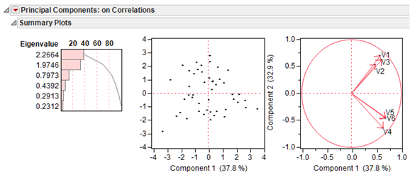
The initial summary plots are a graphical summary of the principal components extracted from the Prosocial Behavior data.

The chart on the left shows a Pareto chart of the eigenvector values used to compute the principal components with the first (largest) at the top. Recall that an eigenvalue is the amount of variance captured by a given component and is used to compute weights for computing the principal component. Eigenvalues are discussed again later.

The scatterplot in the middle of Figure 14.4 plots the computed score values of principal component 2 (PC2) versus Component 1 (PC1). Score values are defined mathematically in the previous section, “How Principal Components Are Computed.” There is a red triangle option to see a matrix of score plots for each pair of principal components. The red triangle option Save Principal Components creates six new columns in the data table that list the PC scores.

The plot on the right is called a Loadings plot. The loadings can give meaning to the scores. They define the orientation of the principal components plane with respect to the original X variables. The loadings define how the variables are linearly combined to form scores. They are the weights in the linear combinations.

The initial loadings plot can show which variables are influential in the bivariate plot space for PC1 and PC2 and how the variables are correlated. The grouping of the correlated variables is seen to be the same as previously shown in the correlation table. The distance from the origin also displays information; variables farther from the origin have greater influence on the model.

Figure 14.4: Initial Plots from the Principal Components Platform

In principal component analysis, the number of components extracted is equal to the number of variables being analyzed. Because six variables are analyzed in the present study, six components are extracted.

The first component can be expected to account for a large amount of the total variance. Each succeeding component then accounts for progressively smaller amounts of variance. Although a large number of components can be extracted in this way, only the first few components are sufficiently important to be retained for interpretation.

The analysis begins with the eigenvalue table. An eigenvalue represents the amount of variance captured by a given component. The row labeled Eigenvalue shows each component’s eigenvalue. The first column gives information about the first principal component, the second column gives information about the second component, and so forth.

The eigenvalue for PC1 is 2.2664 and the eigenvalue for PC2 is 1.9746. Note that the eigenvalue of each successive component is less than the previous one. This pattern is consistent with the statement made earlier that the first components tend to account for relatively large amounts of variance whereas the later components account for relatively smaller amounts.

Figure 14.5: Results of Principal Components Analysis

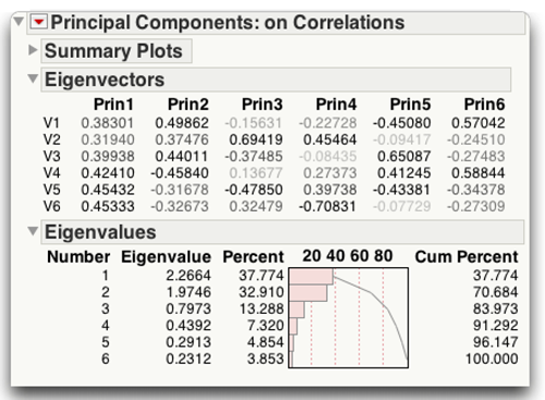
The “How Principal Components Are Computed” defined a principal component as a linear combination of optimally weighted observed variables. These optimal weights are such that no other set of weights can produce principal components that successively account for more variation.

The Eigenvectors table in the Principal Components report (Figure 14.5) gives these optimal weights. The principal components are computed on standardized values. Suppose Sn represents the standardized values of Vn. That is,

Then, the formulas for the first two principal components (using rounded coefficients) are

C1 = 0.383(S1) + 0.319(S2) + 0.399(S3) + 0.424(S4) + 0.454(S5) + 0.453(S6)

C2 = 0.499(S1) + 0.375(S2) + 0.440(S3) – 0.458(S4) – 0.317(S5) – 0.327(S6)

Using the eigenvalues, six principal component scores can be computed for each participant in the study.

Step 2: Determine the Number of Meaningful Components

The number of components extracted is equal to the number of variables analyzed. In general, you expect that only the first few components account for meaningful amounts of variance and that the later components tend to account for only trivial variance. The next step of the analysis is to determine how many meaningful components should be retained for interpretation.

This section describes the following criteria that can be used in making this decision:

• the eigenvalue-one criterion
• the scree test
• the proportion of variance accounted for

Retain Components Based on the Eigenvalue-One Criterion

In principal component analysis, one of the most commonly used criteria for solving the number-of-components problem is the eigenvalue-one criterion, also known as the Kaiser-Guttman criterion (Kaiser, 1960). With this approach, you retain and interpret any component with an eigenvalue greater than 1.00.

The rationale for this criterion is straightforward. Each observed variable contributes one unit of variance to the total variance in the data. Any component that displays an eigenvalue greater than 1.00 accounts for a greater amount of variance than had been contributed by one variable. Such a component therefore accounts for a meaningful amount of variance and is worthy of further consideration.

On the other hand, a component with an eigenvalue less than 1.00 accounts for less variance than contributed by one variable. The purpose of principal component analysis is to reduce a number of observed variables into a relatively smaller number of components. This cannot be effectively achieved if you retain components that account for less variance than had been contributed by individual variables. For this reason, components with eigenvalues less than 1.00 are viewed as trivial and are not retained.

The eigenvalue-one criterion has a number of positive features that contribute to its popularity. Perhaps the most important reason for its widespread use is its simplicity. You do not make subjective decisions but merely retain components with eigenvalues greater than one.

Further, it has been shown that this criterion often results in retaining the correct number of components, particularly when a small to moderate number of variables are analyzed and the variable communalities are high. Stevens (1986) reviews studies that have investigated the accuracy of the eigenvalue-one criterion and recommends its use when fewer than 30 variables are being analyzed and communalities are greater than 0.70, or when the analysis is based on more than 250 observations and the mean communality is greater than 0.59.

However, there are a number of problems associated with the eigenvalue-one criterion. This approach sometimes leads to retaining the wrong number of components under circumstances that are often encountered in research such as when many variables are analyzed or when communalities are small. Also, the mindless application of this criterion can lead to retaining a certain number of components when the actual difference in the eigenvalues of successive components is trivial. For example, if component 2 displays an eigenvalue of 1.01 and component 3 displays an eigenvalue of 0.99, then component 2 is retained but component 3 is not. This can mislead you to believe that the third component was meaningless when, in fact, it accounted for almost exactly the same amount of variance as the second component. In short, the eigenvalue-one criterion can be helpful when used judiciously but the thoughtless application of this approach can lead to errors of interpretation.

Figure 14.5 shows the eigenvalues for PC1, PC2, and PC3 are 2.27, 1.97, and 0.80, respectively. Only PC1 and PC2 had eigenvalues greater than 1.00 so the eigenvalue-one criterion leads you to retain and interpret only these two components.

The application of the criterion is fairly unambiguous in this case. The second (and last) component retained displays an eigenvalue of 1.97, which is substantially greater than 1.00. The next component (3) displays an eigenvalue of 0.80, which is much lower than 1.00. In this analysis you are not faced with the difficult decision of whether to retain a component that demonstrates an eigenvalue approaching 1.00. In situations such as this, the eigenvalue-one criterion can be used with confidence.

Retain Components Based on the Scree Test

The scree test (Cattell, 1966) plots the eigenvalues associated with each component and looks for a definitive break in the plot between the components with relatively large eigenvalues and those with small eigenvalues. The components that appear before the break are assumed to be meaningful and are retained for rotation whereas those appearing after the break are assumed to be unimportant and are not retained. Sometimes a scree plot displays several large breaks. When this is the case, you should look for the last break before the eigenvalues begin to level off. Only the components that appear before this last large break should be retained.

The scree test provides reasonably accurate results provided that the sample is large (over 200) and most of the variable communalities are large (Stevens, 1986). However, this criterion has its own weaknesses, most notably the ambiguity that is sometimes displayed by scree plots under typical research conditions. Often, it is difficult to determine exactly where in the scree plot a break exists, or even if a break exists at all. In contrast to the eigenvalue-one criterion, the scree test is usually more subjective.

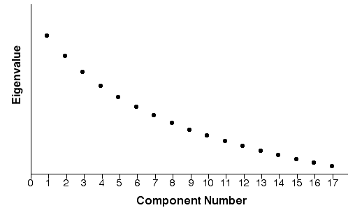
Figure 14.6 presents a fictitious scree plot from a principal component analysis of 17 variables. Notice that there is no obvious break in the plot that separates the meaningful components from the trivial components. Most researchers would agree that components 1 and 2 are likely to be meaningful whereas components 13 to 17 are probably trivial. Scree plots such as this one are common in social science research. This example underscores the qualitative nature of judgments based solely on the scree test. The scree test must be supplemented with additional criteria such as the variance accounted for criterion, described later.

Figure 14.6: Hypothetical Scree Plot with No Obvious Break

A scree plot for the fictitious prosocial data illustrates how this kind of plot can be useful.

Select Scree Plot from the red triangle menu on the Principal Components title bar.

The scree plot in Figure 14.7 shows the component numbers (row numbers) on the horizontal axis and eigenvalues on the vertical axis. Notice there is a small break between components 1 and 2, and a larger break following component 2. The breaks between components 3, 4, 5, and 6 are fairly small. Because the large break in this plot appears between components 2 and 3, the scree test leads you to retain only components 1 and 2.

Figure 14.7: Scree Plot for prosocial Data

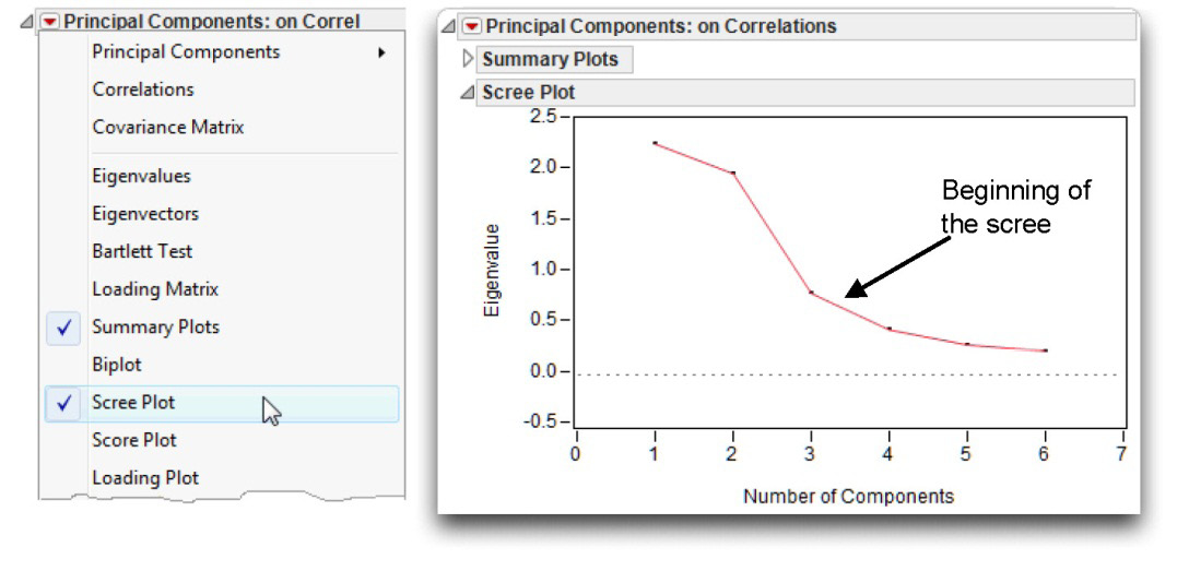
Why is it called a scree test? The word scree refers to the loose rubble that lies at the base of a cliff or glacier. You hope that the scree plot takes the form of a cliff. The eigenvalues at the top represent the few meaningful components, followed by a definitive break (the base of the cliff). The eigenvalues for the trivial components form the scree at the bottom of the cliff.

Retain Components Based on Proportion of Variance Accounted For

A third criterion in choosing the number of principal components to consider involves retaining a component if it exceeds a specified proportion (or percentage) of variance in the data. For example, you might decide to retain any component that accounts for at least 10% of the total variance. This proportion can be calculated with a simple formula:

Or, the initial set of plots show the eigenvalue table and a more detailed report of the eigenvalues is available when you select EigenValues from the red triangle menu (see Figure 14.8).

In principal component analysis, the eigenvalues sum to the number of variables being analyzed because each variable contributes one unit of variance to the analysis. The proportion of variance captured by each component is printed in the eigenvalue table in the report column called Percent.

You can see that the first component accounts for 37.774% of the total variance, the second component accounts for 32.910%, the third component accounts for 13.288%, and the fourth component accounts for 7.320%. Assume that you decide to retain any component that accounts for at least 10% of the total variance in the data. For the present results this criterion causes you to retain components 1, 2, and 3. Notice that this results in retaining more components than would be retained with either the eigenvalues-one criteria or the scree test.

Figure 14.8: Eigenvalues Report for prosocial Example

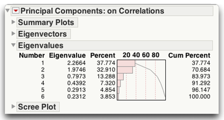
An alternative criterion is to retain enough components so that the cumulative percent of variance accounted for is equal to some minimal value. For example, components 1, 2, 3, and 4 account for approximately 38%, 33%, 13%, and 7% of the total variance, giving. This means that the cumulative percent of variance accounted for by components 1, 2, 3, and 4 is 91%.

When researchers use the cumulative percent of variance accounted for as the criterion for solving the number-of-components problem, they usually retain enough components so that the cumulative percent of variance accounted for is at least 70% (and sometimes 80%). Retaining only components 1 and 2 accounts for 70.6842% of the variance, as seen in the report column labeled Cum Percent. Each value in that row indicates the percent of variance accounted for by the present component as well as all preceding components. The entry for component 3 is 83.9725, which means that approximately 84% of the variance is accounted for by the components 1, 2, and 3.

The proportion of variance criterion has a number of positive features. For example, in most cases, you do not want to retain a group of components that account for only a fraction of variance in the data (say, 30%). Nonetheless, the critical values discussed earlier (10% for individual components and 70% to 80% for the combined components) are arbitrary. Because of these and related problems, this approach has sometimes been criticized for its subjectivity (Kim and Mueller, 1978b).

Recommendations

Given the preceding options, what procedure should you follow in solving the number-of-components problem? First, look at the eigenvalue-one criterion. Use caution if the break between the components with eigenvalues above 1.00 and those below 1.00 is not clear-cut.

Next, perform a scree test and look for obvious breaks in the eigenvalues. Because there is often more than one break in the scree plot, it might be necessary to examine two or more possible solutions.

Next, review the amount of variance accounted for by each individual component. You probably should not rigidly use some specific but arbitrary cutoff point such as 5% or 10%. Still, if you are retaining components that account for as little as 2% or 3% of the variance, it is wise to take a second look at the solution and verify that these latter components are truly of substantive importance. In the same way, it is best if the combined components account for at least 70% of the cumulative variance. If the components you choose to retain account for less than 70% of the cumulative variance, it might be prudent to consider alternative solutions that include a larger number of components.

Step 3: Rotate to a Final Solution

Ideally, you want to review the correlations between the variables and components, and use this information to interpret the components. That is, you want to determine what construct seems to be measured by PC1, what construct seems to be measured by PC2, and so forth. When more than one component is retained in an analysis, the interpretation of an unrotated pattern can sometimes be difficult. To facilitate interpretation, you can perform an operation called a rotation. A rotation is a linear transformation performed on the principal components for the purpose of making the solution easier to interpret.

The menu on the Principal Components title bar has the Factor Analysis command. When you choose this command, the dialog shown here prompts for Factoring Method and Prior Communality choices, and the number of factors to rotate. For this example, use the Principal Components results for both the Factoring method and Prior Communalities.

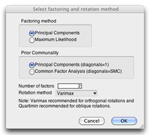
This fictitious example is designed to have two distinct factors so enter 2 as the number of factors to rotate.

The rotation method menu has many options, but the most familiar method is the default varimax rotation (Kaiser, H. F. 1960). A varimax rotation is an orthogonal rotation, which means that the rotated components are uncorrelated. Compared to other types of rotations, a varimax rotation tends to maximize the variance of a column of the factor pattern matrix (as opposed to a row of the matrix). This rotation is a commonly used orthogonal rotation in the social sciences. Figure 14.9 shows the results of the varimax rotation.

Note: Using a principal components analysis, retaining components with eigenvalues greater than 1, and then performing a varimax rotation to produce uncorrelated factors is called a little jiffy factor analysis (Kaiser, 1970). Thus, the following steps and discussion apply equally well to factor analysis as principle component analysis.

Figure 14.9: Factor Rotation Report for Principal Component Analysis

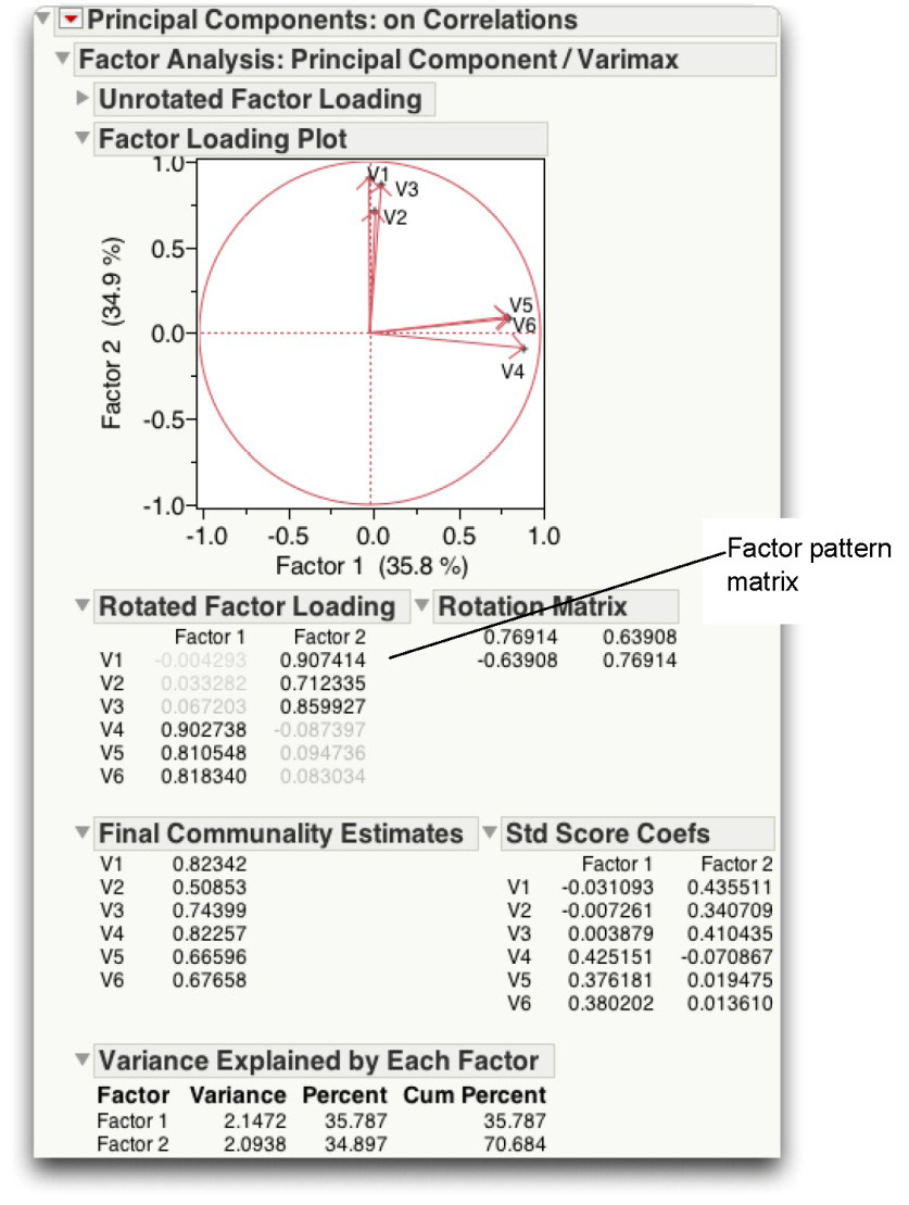
Step 4: Interpret the Rotated Solution

A rotated solution helps you determine what is measured by each of the retained components (2 in this example). You want to identify the variables that exhibit high loadings for a given component, and determine what these variables share in common.

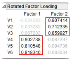
At this stage, the first decision to be made is to decide how large a factor loading must be to be considered “large.” Stevens (1986) discusses some of the issues relevant to this decision and even provides guidelines for testing the statistical significance of factor loadings. Given that this is an introductory treatment of principal component analysis, simply consider a loading to be “large” if its absolute value exceeds 0.40. Note in the Rotated Factor Loading table, small loading values are dimmed.

A. Read the loading values for the first variable.

The Rotated Factor Loading table lists each variable (V1–V6) and shows the loading values for two factors. The loading values for V1 are –0.004293 and 0.907414. V1 has a small loading (shows as dimmed) on the first factor and a large loading (greater than 0.40) on the second factor. If a given variable has a meaningful loading on more than one component, ignore it in your interpretation. In this example, V1 loads on only one factor so you retain this variable.

B. Repeat this process for the remaining variables and eliminate any variable that loads on more than one component.

In this analysis, none of the variables have high loadings on more than one component, so none have to be deleted from the interpretation. In other words, there are no complex items.

C. Review all of the variables with high loadings on PC1 to determine the nature of this component.

From the rotated factor pattern, you can see that only items 4, 5, and 6 (V4–V6) load on the first component. It is now necessary to turn to the questionnaire itself and review the content in order to decide what a given component should be named. What do questions 4, 5, and 6 have in common? What common construct do they appear to be measuring?

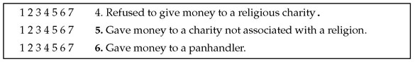
For illustration, the questions being analyzed in the present case are reproduced here. Read questions 4, 5, and 6 (V4–V6) to see what they have in common.

Questions 4, 5, and 6 all seem to deal with “giving money to those in need.” It is therefore reasonable to label component 1 the “financial giving” component.

D. Repeat this process to name the remaining retained components.

In the present case, there is only one remaining component to name—component 2. This component has high loadings for questions 1, 2, and 3 (V1–V3). Each of these items seems to deal with helping friends, relatives, or other acquaintances. It is therefore appropriate to name this the “helping others” component.

Step 5: Create Factor Scores or Factor-Based Scores

Once the analysis is complete, it is often desirable to assign scores to participants to indicate where they stand on the retained components. For example, the two components retained in the present study can be interpreted as “financial giving” and “helping others.” You might want to now assign one score to each participant to indicate that participant’s standing on the “financial giving” component and a different score to indicate that participant’s standing on the “helping others” component. With this done, these component scores could be used either as predictor variables or as response variables in subsequent analyses.

Before discussing the options for assigning these scores, it is important to first draw a distinction between factor scores versus factor-based scores.

• In principal component analysis, a factor score (or component score) is a linear composite of the optimally weighted observed variables.
• A factor-based score is a linear composite of the variables that demonstrates meaningful loadings for the component in question. In the preceding analysis, items 4, 5, and 6 demonstrated meaningful loadings for the “financial giving” component. Therefore, you could calculate the factor-based score on this component for a given participant by simply adding together a participant’s responses to items 4, 5, and 6. The observed variables are not multiplied by optimal weights before they are summed.

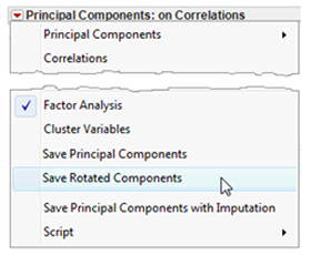
Computing Factor Scores

You can save each participant’s factor scores for the two components as new columns in the prosocial behavior data table using the Save Rotated Components command found in the menu on Principal Components title bar report. This command multiplies participant responses to the questionnaire items by the optimal weights given in the principal component analysis and sums the products. This sum is a given participant’s score on the component of interest. Remember that a separate equation with different weights is developed for each retained component. The two sets of scores saved in the data table ate named Factor1 and Factor2.

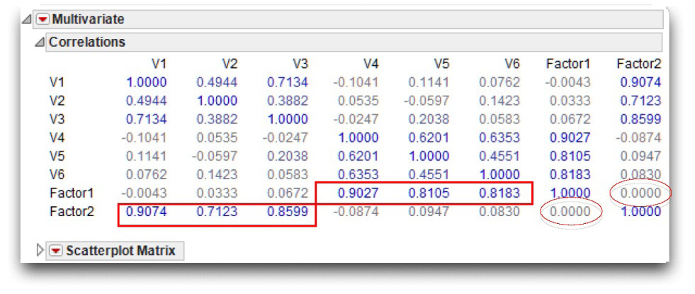
To see how these factor scores relate to the study’s original observed variables, look at the correlations between the factor scores and the original variables.

Choose Multivariate Methods > Multivariate from the Analyze menu.

Select V1–V6 and the new variables Factor1 and Factor2 as analysis variables. Click OK on the Multivariate launch dialog to see the correlations shown in Figure 14.10.

The correlations between Factor1 and Factor2 and the original observed variables appear towards the bottom of the multivariate report. You can see that the correlations between Factor1 and V1 to V6 are identical to the factor loadings of V1 to V6 on Factor1 shown as the Rotated Factor Pattern table shown previously. This makes sense, as the elements of a factor pattern (in an orthogonal solution) are simply correlations between the observed variables and the components themselves. Similarly, you can see that the correlations between Factor2 and V1 to V6 are also identical to the corresponding factor loadings from the Rotated Factor Pattern table.

Of special interest is the correlation between Factor1 and Factor2. Notice the observed correlation between these two components is zero. This is as expected because the rotation method used in the principal component analysis is the varimax method, which produces orthogonal (uncorrelated) components.

Figure 14.10: Correlations between Rotated Factors and Original Variables

Computing Factor-Based Scores

A second (and less sophisticated) approach to scoring involves the creation of new variables that contain factor-based scores instead of true principal component scores. A variable that contains factor-based scores is sometimes called a factor-based scale.

Although factor-based scores can be created in a number of ways, the following method has the advantage of being relatively straightforward and is commonly used.

To calculate factor-based scores for component 1, first determine which questionnaire items had high loadings on that component.

For a given participant, add together that participant’s responses to these items. The result is that participant’s score on the factor-based scale for component 1.

Repeat these steps to calculate each participant’s score on the remaining retained components.

You can do this in JMP by creating two new columns in the current data table (the table used to create rotated components). You have looked at the factor loadings and found that survey items 4, 5, and 6 loaded on component 1 (“financial giving” component) and items 1, 2, and 3 loaded on component 2 (“helping others” component).

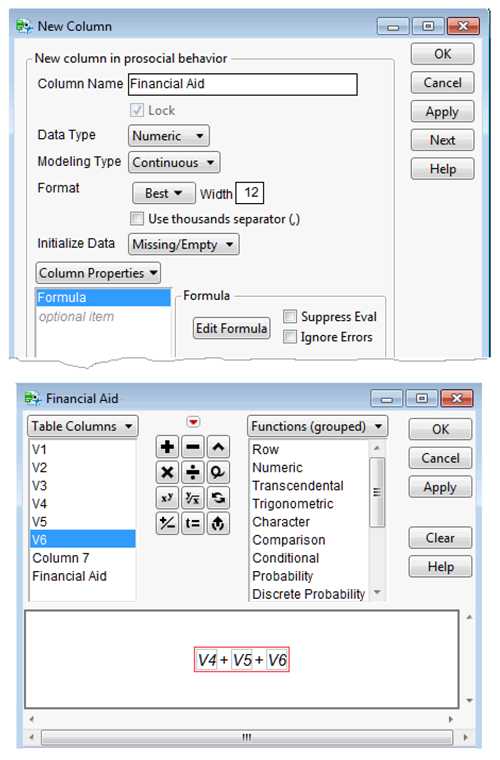
To create the factor-based scores, create two new variables in the prosocial behaviour.jmp data table and name them financial aid and helping others.

Choose New Column from the Cols menu. When the New Column dialog appears, enter Financial Aid as the column name.

Click New Property from the New Column dialog, and then select Formula from its menu.

Use the Formula Editor to create the formula to compute the factor-based score for ". Click V4 in the list of variables, and then click the plus operator. Click V5, then click the plus operator, and finally click V6.

Click OK on the Formula Editor.

Figure 4.11 shows the New Column dialog, the formula editor, and its formula to compute the factor-based scores for the first component.

Follow the same steps to create the second new column called helping others, but use the column V1 + V2 +V3 to compute the factor-based scores for the second component.

Here is a shortcut method to create a new column and a formula:

• To create a new column, double-click anywhere in the empty area of the data table to the right of the existing columns.
• Highlight the column name area and type a new name (Helping Others).
• To see a column editor for the new column, right-click in the column heading area and choose Formula from the menu that appears.
• Enter the formula as described previously, and then close the Formula Editor.

Figure 14.11: New Column Dialog and Formula Editor

The first variable, called Financial Aid, lists each participant’s factor-based score for financial giving. The second variable, called Helping Others, lists each participant’s factor-based score for helping others. These new variables could be used as predictor variables in subsequent analyses.

However, the correlation between Financial Aid and Helping Others is not zero, unlike the factor scores, Factor 1 and Factor 2. This is because Factor 1 and Factor 2 are true principal components (created in an orthogonal solution) and are optimally weighted equations to be uncorrelated. In contrast, Financial Aid and Helping Others are not true principal components. They are variables based on factors identified by the factor loadings of a principal component analysis. These factor-based scores do not use optimal weights that ensure orthogonality.

Recoding Reversed Items Prior to Analysis

It is generally best to recode any reversed items before conducting any of the analyses described here. In particular, it is essential that reversed items be recoded prior to the program statements that produce factor-based scales. For example, the three questionnaire items that assess financial giving appear again here.

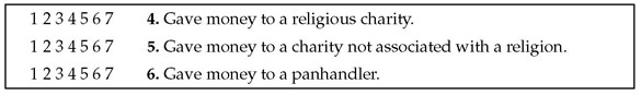
None of the previous items are reversed. With each item, a response of 7 indicates a high level of financial giving. However, in the following list item 4 is a reversed item—a response of 7 indicates a low level of giving.

If you perform a principal component analysis on responses to these items, the factor loading for item 4 would most likely have a sign that is the opposite of the sign of the loadings for items 5 and 6. That is, if items 5 and 6 had positive loadings, item 4 would have a negative loading. This complicates the creation of a factor-based scale. You would not want to sum these three items as they are presently coded. First, it is necessary to reverse item 4. You can do this in the JMP table by creating another formula based variable, call it V4 new, using the formula

8 – V4

Values of this new version of V4 are 8 minus the value of the old version of V4. A participant whose score on the old version of V4 is 1 has a value of 7 (8 – 1 = 7) on the new version, whereas someone who has a score of 7 now has a score of 1 (8 – 7 = 1). Note that the constant (8) used to create the new values is 1 greater than the number of possible responses to an item. If you use a 4-point response format, then the constant is 5. If you use a 9-point scale, then the constant is 10.

If you have prior knowledge about which items are will show reversed component loadings in your results, it is best to recode them before the analysis. This makes interpretation of the components more straightforward because it eliminates significant loadings with opposite signs from appearing on the same component.

Step 6: Summarize Results in a Table

For reports that summarize the results of your analysis, it is desirable to prepare a table that presents the rotated factor pattern. When analyzed variables contain responses to questionnaire items, it can be helpful to actually reproduce the questionnaire items within this table. This is done in Table 14.4.

Table 14.4: Rotated Factor Pattern and Final Communality Estimates from Principal Component Analysis of Prosocial Orientation Inventory

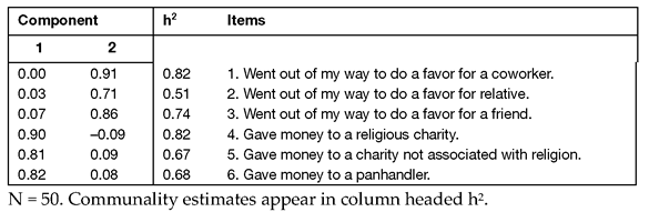
The final communality estimates from the analysis are presented under the heading h2 in the table. Often, the items that constitute the questionnaire are so lengthy or the number of retained components is so large that it is not possible to present the factor pattern, the communalities, and the items themselves in the same table. In such situations, it might be preferable to present the factor pattern and communalities in one table and the items in a second table (or in the text of the paper). Shared item numbers can then be used to associate each item with its corresponding factor loadings and communality.

Step 7: Prepare a Formal Description of Results for a Paper

The preceding analysis could be summarized in the following way:

Principal component analysis was applied to responses to the 6-item questionnaire. The principal axis method was used to extract the components, and was then followed by a varimax (orthogonal) rotation.
Only the first two components exhibited eigenvalues greater than 1; results of a scree test also suggested that only the first two components were meaningful. Therefore, only the first two components were retained for rotation. Combined, components 1 and 2 accounted for 71% of the total variance.
Questionnaire items and corresponding factor loadings are presented in Table 14.4. In interpreting the rotated factor pattern, an item was said to load on a given component if the factor loading was .40 or greater for that component and less than 0.40 for the other component. Using these criteria, three items were found to load on the first component, which was subsequently labeled “financial giving.” Three items also loaded on the second component, which was labeled “helping others.”

Summary

Principal component analysis is an effective procedure for reducing a number of observed variables to a smaller number of variables that account for most of the variance in a set of data. This technique is particularly useful when you need a data reduction procedure that makes no assumptions concerning an underlying causal structure responsible for correlation in the data. When such an underlying causal structure can be envisioned, it might be more appropriate to analyze the data using exploratory factor analysis.

Appendix: Assumptions Underlying Principal Component Analysis

Because a principal component analysis is performed on a matrix of Pearson correlation coefficients, the data should satisfy the assumptions for this statistic. These assumptions were described in detail in Chapter 6, “Measures of Bivariate Association,” and are briefly reviewed here:

Continuous numeric measurement

All variables should be assessed on continuous numeric measurements.

Random sampling

Each participant contributes one score on each observed variable. These sets of scores should represent a random sample drawn from the population of interest.

Linearity

The relationship between all observed variables should be linear.

Bivariate normal distribution

Each pair of observed variables should display a bivariate normal distribution (they should form an elliptical point cloud when plotted).

References

Cattell, R. B. 1966. “The Scree Test for the Number of Factors.” Multivariate Behavioral Research, 1, 245–276.

Clark, L. A., and Watson, D. 1995. “Constructing Validity: Basic Issues in Objective Scale Development.” Psychological Assessment, 7, 309–319.

Gabriel, R. K. 1982. “Biplot.” Encyclopedia of Statistical Sciences, Volume I, eds., N. L. Johnson and S. Kotz. New York: John Wiley & Sons.

Kaiser, H. F. 1958. “The Varimax Criterion for Analytic Rotation in Factor Analysis.” Psychometrica, 23, 187–200.

Kaiser, H. F. 1960. “The Application of Electronic Computers to Factor Analysis.” Educational and Psychological Measurement, 20, 141–151.

Kaiser, H. F. 1970. “A Second Generation Little Jiffy.” Psychometrika, 35, 401–415.

Kim, J. O., and Mueller, C. W. 1978a. Introduction to Factor Analysis: What It Is and How to Do It. Beverly Hills, CA: Sage.

Kim, J. O., and Mueller, C. W. 1978b. Factor Analysis: Statistical Methods and Practical Issues. Beverly Hills, CA: Sage.

O’Rourke, N., and Cappeliez, P. 2002."Development and Validation of a Couples Measure of Biased Responding: The Marital Aggrandizement Scale." Journal of Personality Assessment, 78, 301–320.

Rummel, R. J. 1970. Applied Factor Analysis. Evanston, IL: Northwestern University Press.

Rusbult, C. E. 1980. “Commitment and Satisfaction in Romantic Associations: A Test of the Investment Model.” Journal of Experimental Social Psychology, 16, 172–186.

Spector, P. E. 1992. Summated Rating Scale Construction: An Introduction. Newbury Park, CA: Sage.

Stevens, J. 1986. Applied Multivariate Statistics for the Social Sciences. Hillsdale, NJ: Lawrence Erlbaum.

Streiner, D. L. 1994. “Figuring Out Factors: The Use and Misuse of Factor Analysis.” Canadian Journal of Psychiatry, 39, 135–140.