
 3
3
Overview
This chapter covers the basics of data input in JMP. Topics include simple input such as keying in data, how to copy and paste data, reading simple and complex raw text files, reading SAS data sets, and reading data from other external files. Also, this chapter includes an overview of characteristics of JMP data including data created by formulas.
If you are familiar with JMP, use this chapter to review, and then move on to the subsequent data analysis chapters.
Read Data into JMP from Other Files
Compute Column Values with a Formula
Structure of a JMP Table
Before any analysis work can be done, data must be in the form of a JMP data table. The next section talks about creating new tables. This section assumes there is an existing JMP table. To open an existing table, double-click on the JMP table icon, or use the Open command on the File menu and navigate to the table you want to open.
The Open File dialog in JMP is similar to those in other applications. Notice that in the Open File dialog JMP can open many different kinds of file types, including SAS files, Microsoft Excel files, text files, and others.
An open JMP table called social survey is shown in Figure 3.1 with annotations of the components you need to know about. These features are discussed below.
Figure 3.1: Data Table Elements
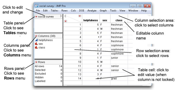
The data table is divided into two parts: the left side of the table consists of three panels, and the right side of the table is the data grid.
- The Table panel, at the left top of the table, shows the data table name; the icon on its title bar accesses the Tables main menu, and has several additional specialized commands.
- The Columns panel lists the columns in the table; the icon in its title bar accesses the Cols main menu.
- The Rows panel shows the total number of rows and summarizes characteristics assigned to rows; the icon on its title bar accesses the Rows main menu.
- The data grid holds the data values in a spreadsheet fashion.
Using the Data Table Panels
The panels on the left side of the data grid show overall information about the data table and give quick access to the Tables, Rows, and Columns main menu commands. Drag the divider that separates the panels from the data grid to make the panels wider or narrower. The data table panels and main menu commands are described briefly here and discussed in more detail later in this chapter.
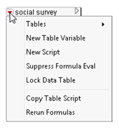
The Table Panel
The Table panel is at the top of the data table’s panels. The icon on the Table panel title bar accesses commands for manipulating the table and creating and storing table information. The first command (Tables) is the same as the Tables command on the main menu. Table panel commands let you document the table with special table variables, lock the table, create new scripts (JMP programs) for the table, attach scripts to the table, edit and run attached scripts, and determine when formulas should be evaluated.
The Columns Panel
The Columns panel lists the columns (also called variables) in the data table in the order they appear from left to right in the data grid. You can rearrange the columns by grabbing and dragging the column names up or down in the Columns panel. The Columns panel title bar shows the total number of columns and the number of columns that are selected (highlighted). The “Selecting (Highlighting) Rows and Columns” section later in this chapter gives details about selecting rows and columns. The icon on the Columns panel title bar accesses the Columns main menu commands.
To the left of each column name is an icon that indicates the modeling type of each variable. The modeling type of a variable gives information about how to analyze the variable to the JMP analysis platforms. Details about modeling types are discussed later in this chapter in the “Data Types and Modeling Types” section.
The Rows Panel
The Rows panel tells how many rows are in the table and gives information about certain row states. Rows can be selected, excluded, hidden, and labeled. The Exclude/Unexclude, Hide/Unhide, and Label/Unlabel commands assign row states and are found on the Rows main menu or the Rows menu on the Rows panel title bar. These commands affect only selected (highlighted) rows.
To select (highlight) rows, click in the row number area to the left of the data in the data grid. The row number area is then highlighted, and the number of selected rows is displayed in the Rows panel. To select multiple rows, drag down the rows (or shift-click on the first and last row you want to select). To make a noncontiguous selection, control-click (![]() -click on the Macintosh) on the rows to be selected.
-click on the Macintosh) on the rows to be selected.
Using the Data Grid
The data grid is the set of rows and columns that contain the data you want to analyze. A data cell is the intersection of a row and a column. If the column does not have a formula that computes its values, and isn’t locked, you can enter or edit data in a cell.
Both rows and columns can be rearranged by dragging them in the data grid. To move one or more rows or columns, first select them, and then click and drag to the position in the table you want the selected items to precede. Alternatively, the Move Rows command on the Rows menu and the Reorder Columns command on the Columns menu operate on selected rows and columns.
The upper-left corner of the data table offers several useful table actions.
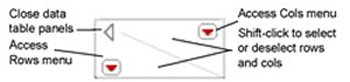
- To select all rows or all columns at the same time, shift-click in the triangular area above the row numbers or next to the column names. Likewise, to deselect all rows or columns, click in the appropriate triangular area in the upper-left corner of the data grid.
- The red icons access the Rows and Columns main menus. You can also see these menus by using a right click (control-click on the Macintosh) anywhere in the triangular rows and columns areas.
- The disclosure icon in the upper-left corner of the data grid hides the data table panels section, leaving only the data grid showing.
The following sections discuss creating a data table and entering different kinds of data.
JMP Tables, Rows, and Columns
The previous section, “Structure of a JMP Table,” describes the components of a JMP data table and briefly talks about the rows and columns in a table. The current section expands on creating and using rows and columns, describes types and properties of data, and shows how to get data into JMP.
Data for the examples are in the form of a JMP table. You can access the example tables from the author page for this book at support.sas.com/authors.
To open an example JMP table, double-click on its icon or use the Open command on the File menu. Then proceed with the examples. However, to process your own data, they must be in a JMP data table.
Create a New Table
Follow these steps to create and name a new data table, and enter data.
![]() Choose the New command from the File menu. A new JMP table appears with one column, called Column 1, showing. Add additional columns by clicking anywhere in the empty part of the data grid.
Choose the New command from the File menu. A new JMP table appears with one column, called Column 1, showing. Add additional columns by clicking anywhere in the empty part of the data grid.

![]() Give the new table a name. The default name, Untitled, is displayed in the upper-left corner of the table. When you double-click on the table name it becomes editable, and you can enter a new table name. Alternatively, you can use the Save As command from the File menu and name the table in the Save As dialog.
Give the new table a name. The default name, Untitled, is displayed in the upper-left corner of the table. When you double-click on the table name it becomes editable, and you can enter a new table name. Alternatively, you can use the Save As command from the File menu and name the table in the Save As dialog.
![]() Click any cell in the data grid to see a cursor for typing data. Enter a value and press the Enter key to move the cursor to the next row.
Click any cell in the data grid to see a cursor for typing data. Enter a value and press the Enter key to move the cursor to the next row.
![]() To edit or delete cell values, drag over them in the cell and retype the data, or press the Delete key to erase them.
To edit or delete cell values, drag over them in the cell and retype the data, or press the Delete key to erase them.
![]() Type data into cells as you would in any spreadsheet.
Type data into cells as you would in any spreadsheet.
Double-click in the empty areas of a data grid to create new rows and columns. Or, use the Add Rows command on the Rows menu to create a specified number of new rows. Use the New Column or Add Multiple Columns commands on the Cols menu to add new columns. To name a new column, click on the column name at the top of the column and begin typing. You can also modify a column name and other column characteristics with the Column Info command in the Cols menu.
Note: You can drag the lines between columns to change the column width in the table, and drag to make the rows area wider or narrower.
Selecting (Highlighting) Rows and Columns
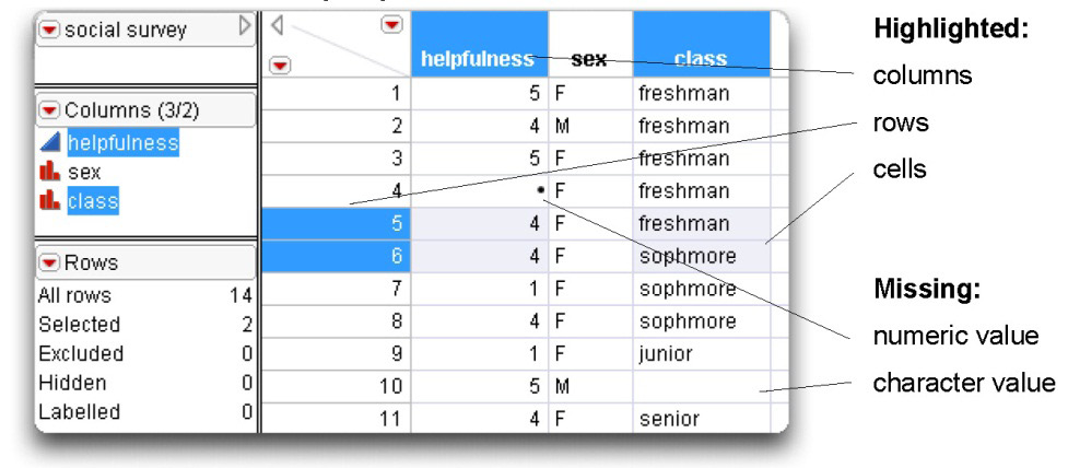
Many commands on the Rows menu and Cols menu only apply to selected rows and columns. Editing values takes place in selected cells. Figure 3.2 shows examples of highlighted rows, columns, and cells.
- To select a row, click on the space to the left of the row number.
- To select a column, click on the space at the top of the column or on the column name in the Columns panel.
- Click in a cell to select it for data entry or data editing.
Figure 3.2: Data Table with Highlighted Rows and Columns
Select multiple rows by dragging up or down the row space to the left of the row numbers. Likewise, select multiple columns by dragging across the space at the top of the columns or on the column names in the Columns panel. You can select rows or columns that are not next to each other (noncontiguous) by using control-click (command-click on the Macintosh).
To deselect (unhighlight) all selected rows, click on the triangular area in the upper left of the data grid, above the row numbers. Likewise, to deselect all selected columns, click on the triangular area in the upper left of the data grid next to the column names. To deselect a single row or column, control-click on the row or column space.
You can also select multiple rows and columns by dragging across the cells that form the intersection of those rows and columns. Use control-click to drag across noncontiguous cells.
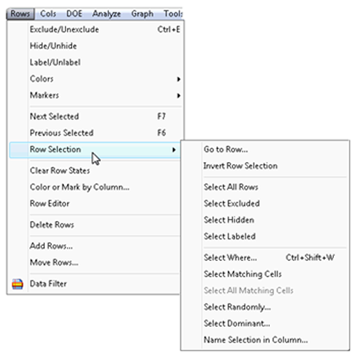
You can also select specific subsets of rows using the Row Selection command on the Rows menu (see Figure 3.3). Row Selection has a list of subcommands that do almost any kind of selection you need. Several of the most commonly used selection commands are as follows:
Go to Row deselects all currently selected rows, and then moves the cursor to the row you specify and selects it.
Invert Row Selection reverses the selection status of all rows.
Select All Rows selects all rows.
Select Randomly randomly selects the proportion of rows or sample size you specify.
Figure 3.3: Row Selection Dialog
Note: The data table and all analyses on that table are linked. For example, when you click on a histogram bar, the corresponding rows in the data table are then highlighted. Selecting points in a plot also highlights them in the data table.
Creating and Deleting Columns
You can add columns as needed to a JMP table in the following ways:
- Double-click anywhere in the empty grid area to the right of the current columns.
- Use the New Column command on the Cols menu. This command displays the New Column dialog, shown in Figure 3.4, for naming the column and assigning column properties (described later).
- Use the Add Multiple Columns command on the Cols menu. This method of adding columns lets you add any number of sequentially numbered columns with a naming prefix you specify, and lets you position them anywhere in the table. All columns created this way have the same data type (character or numeric).
- Duplicate an existing column. You can drag a column to change its position by highlighting and dragging the column name at the top of the data grid or in the Columns panel. To duplicate a column, highlight the column in the data grid, press the Control key (Option key on the Macintosh,) and drag to a new position.
To change the column name from the default, Column 1 (or to change any column’s name), highlight the column, and then type a name that describes the column values. Or, highlight the column and select Column Info from the Cols menu. Enter a new name in the Name text box in the dialog. Other properties of data are discussed later in this chapter.
To delete one or more columns, highlight them and choose Delete Columns from the Cols menu.
Note: By default, new columns created by double-clicking in the data grid are numeric and accept only numeric data. If you enter alphabetic or special characters, a message asks if you want to change the column to a character column or retype the data.
Creating and Deleting Rows
Whenever you double-click in a cell beneath the current row and then press the Enter key, new empty rows form down to the position of the cursor. Click in any cell to begin entering data.
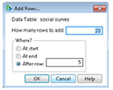
You can also create rows with the Add Rows command on the Rows menu. Add Rows displays the dialog shown here, which lets you enter the number of rows you specify either at the start of the table, at the end of the table, or after the row number you enter to specify where you want the new rows to begin.
Use the Delete Rows command on the Rows menu to delete one or more selected rows.
Data Types and Modeling Types
Data types, modeling types, and other properties are characteristics of columns in the data grid. Columns of data are also called variables.
The Column Info dialog gives all the characteristics and properties of a column. To see the Column Info dialog for a specific column, highlight the column in the data table (click on the space at the top of the column) and choose Column Info from the Cols menu (see Figure 3.4).
The columns in a JMP data table hold different kinds of data, to be used in different ways. The kind of data in a column is called its data type. Data can be any numeric value, alphabetic characters, special keyboard characters, and row state values that JMP creates when you request them. Most of the examples in this book use numeric and character data.
Every column also has a modeling type. The modeling type provides information to the JMP analysis platforms that helps define the analyses. In JMP, it is important to understand modeling types, as well as the relationship between data types and modeling types of variables.
|
Continuous means the data values are numeric only and are analyzed as numeric values. The continuous modeling type includes both the interval and ratio measurement scales. |
|
|
Ordinal means the data may be either numeric or character, but are to be analyzed as categorical values that have an implied order, an ordinal measurement scale. |
|
|
Nominal means the data can have either numeric or character values, have no order, and are analyzed as character or categorical data, a nominal measurement scale. |
A variable with the continuous data type can be assigned any one of the three modeling types. However, a variable with the character data type cannot have a continuous modeling type—it must be assigned as either nominal or ordinal. It is not possible to perform statistical calculations on character values, but it is possible to use numbers as categories. Table 3.1 summarizes the relationship between data types and modeling types.
Table 3.1: Relationship between Data Types and Modeling Types
|
Possible Modeling Type |
||||
|
Continuous |
Ordinal |
Nominal |
||
|
Data Type |
Numeric |
yes |
yes |
yes |
|
Character |
no |
yes |
yes |
|
Assign Properties to Columns
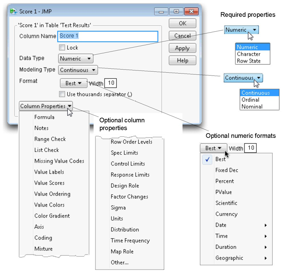
By default, when you create a new column, it is a simple numeric variable with a continuous modeling type. You can change properties of a column or add new properties with the Column Info dialog. Figure 3.4 shows the Column Info dialog for a variable named Score 1 in a data table named Test Results.
The required properties, Data Type and Modeling Type, were discussed in the previous section.
Data Formats
The default format for numeric variables is Best, which displays the data in the best way that the numeric information fits the default field width of 10. However, you can change the field width of both numeric and character variables to be as large as you need.
- Numbers larger than the specified field width are displayed in scientific notation, showing as many decimal places as possible.
- Negative numbers are displayed with a leading minus sign that uses one position in the field width.
- Missing numeric values are displayed as a dot, or period, in the data table.
- Missing character values are displayed as an empty cell in the data table.
There are useful numeric formats (Probability, Currency, Date, Time, and others) that are not needed in this book. For a description of these formats, see Using JMP or the JMP online help facility.
Figure 3.4: Column Options in the Column Info Dialog
Column Formulas
Optionally, columns can have many other properties, but only a few are used in this book. The Column Properties menu on the Column Info dialog (shown above) gives a list of other column properties you can assign to a column. An important additional property used by columns is Formula. The “Compute Column Values with a Formula” section shows how to create a column formula that computes values for that column.
Optional Column Properties
The following are other optional column properties you might find useful when storing data in a JMP table.
Notes
Displays a text box that lets you to enter information about the column. For example, you might want to document a column named Temperature with the phrase, “temperature in degrees Centigrade taken at 12:00 a.m.” Whenever you look at the Column Info dialog, the notes act as column documentation.
Range Check
Lets you enter a range of acceptable values for a numeric column, which limits the values you can enter into the column. If you try to enter a value outside this validation range, a window prompts you to change the value to one within the acceptable range or enter a missing value. If you select Range Check for a column that has values, the Range Check dialog automatically contains the value range using the low and high values found in the column.
List Check
Lets you set up a list of acceptable values for a column. As with Range Check, you can only enter values into the column from the specified list. List Check can be used with either numeric or character columns. If you select List Check for a column that has values, the List Check dialog automatically contains the list of values found in the column.
Value Labels
Lets you display a descriptive label instead of the original value wherever the value appears. For example, the value labels appear in the data table but the original value is not lost. You can double-click in a cell to see the original values. All analyses use the original values.
Many properties are specific to types of analyses not covered in this book. For more details, see Using JMP or the JMP online help facility installed in the JMP Help menu.
Getting Data into JMP
You can enter data into a new JMP table just as you do in any spreadsheet program. When you click on a cell, the cursor becomes an I-beam, and is ready for you to type in data. To edit or delete cell values, drag over them in the cell and retype the data, or press the Delete key to erase them. Two other common ways to fill a JMP table with values is by pasting data from text files, other JMP files, or other applications; and reading data from external files such as SAS, Excel, Word, or other text files.
Copy and Paste Data
The Copy and Paste commands on the Edit menu perform standard operations. Values you copy to the clipboard from other applications can be pasted into JMP, and values copied from JMP can be pasted into other applications.
The Copy command acts on JMP data as follows:
- The entire table is copied to the clipboard when no rows or columns are selected. The same is true if all rows but no columns are selected, or no rows and all columns are selected.
- Copy copies all selected rows if no columns are selected, and all selected columns if no rows are selected.
- When both rows and columns are selected, the subset of values that is the intersection of those rows and columns is copied to the clipboard; select a single row and a single column to copy a single value.
Note: If you use Shift-Copy (Option-Copy on the Macintosh), the column headers as well as the data values are copied to the clipboard. The column headers are displayed when you paste into another application. If you use Shift-Paste to paste the clipboard data into another JMP table, the column headers are preserved in the new table.
Read Data into JMP from Other Files
One common situation is the need to read text data or data from other applications into JMP. Often, the form of the data can be identified by the three-character suffix on the filename, or by the way they are labeled in the Open File dialog list.
Here are a few of the most commonly encountered file types that JMP can read:
- Text Document (txt)
- Text or Data files on Windows (dat)
- Text with comma-delimited values (csv, or cvs)
- SAS versions 5 to 9 (sd2, sd5, sd7, sas7bdat) on Windows—open with the Open command or double-click on file icon to open without dialog
- SAS version 6 (sas7, bdat, ssci, ssd01, sadeb$data) on Macintosh—open with the Open command or double-click on file icon to open without dialog
- SAS Transport files (xpt, stx)
- Microsoft Excel (xls)—use Open command
If a JMP file, Excel file, or SAS file is visible, you can double-click on the file icon to open it directly, instead of using the Open File dialog. If a text or data file has spaces or tab-delimited fields, the Open File dialog often opens them without needing further information.
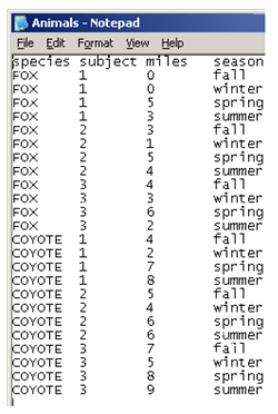
However, a common situation occurs when you have text data with other field delimiters, and variable or column names in the first line of the text file. If the Import/Export preferences are not set to interpret this kind of file, you must provide further information about the file to open it. The file called Animals.txt is an example of raw text data. To see this data in raw form, open it with your system application called Notepad on Windows or TextEdit on the Macintosh. The figure shown here is an illustration of how simple text data appears. You can access this text file from the author page for this book at support.sas.com/authors.
To give information to JMP about how to open this text file, do the following:
![]() Select File > Open and navigate to the Animals.txt file found on the author page for this book to see the dialog in Figure 3.5.
Select File > Open and navigate to the Animals.txt file found on the author page for this book to see the dialog in Figure 3.5.
![]() Select the Data with Preview radio button, which lets you see and change (preview) information about how to read the incoming text file.
Select the Data with Preview radio button, which lets you see and change (preview) information about how to read the incoming text file.
Figure 3.5: Open Data File Dialog Showing Text Files Only
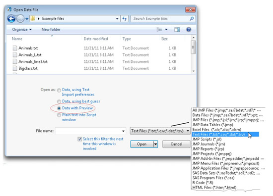
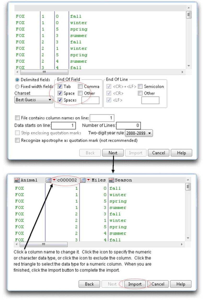
- Select the Animals.txt table and click Open in the Open Data File dialog. Because you selected the Data with Preview radio button, the Text Import Preview dialog at the top in Figure 3.6 appears.
The dialog reflects the way JMP sees the incoming data by showing the first few rows. In this example, Tab, Space, and Spaces are checked as possible End Of Field delimiters. Fields delimited by either of these characters will be read correctly.
Notice the File contains column names on line checkbox. If the text file contains columns names, use this checkbox to specify the line number that has the column names (usually column 1). Further, you can specify the starting line of the data and the number of lines you want to read.
Click the Next button to see the preview dialog at the bottom in Figure 3.6. If the data in the dialog does not match the incoming data, click Back, change the specifications, and try again.
Figure 3.6: Text Import Preview Dialog
Compute Column Values with a Formula
Often, you are interested in analyzing values that are defined by several columns. For instance, you might have recorded two scores for each subject in a study, and want to look at improvement in scores. To do this, you could subtract one score from another. The following steps take you through a simple example of computing column values.
![]() Open the data table called Difference.jmp. It has two numeric columns, score1 and score2, and 10 rows. Suppose you want create a new column that has the difference between the two columns as its values.
Open the data table called Difference.jmp. It has two numeric columns, score1 and score2, and 10 rows. Suppose you want create a new column that has the difference between the two columns as its values.
![]() Create a new column, and call it score2−score1 (or any name you like). See the “Creating and Deleting Columns” section for details about creating and naming new columns.
Create a new column, and call it score2−score1 (or any name you like). See the “Creating and Deleting Columns” section for details about creating and naming new columns.
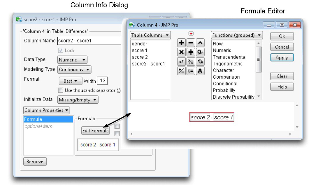
![]() Click at the top of the new column to highlight it, and choose Column Info from the Cols menu to see the Column Info dialog (see Figure 3.7).
Click at the top of the new column to highlight it, and choose Column Info from the Cols menu to see the Column Info dialog (see Figure 3.7).
![]() Select Formula from the New Property menu in the Column Info dialog, as shown in Figure 3.7.
Select Formula from the New Property menu in the Column Info dialog, as shown in Figure 3.7.
The Formula Editor creates a formula that is permanently stored with a specific column. Once a formula is assigned to a column, that column becomes locked, which means you can no longer manually enter values. The column is also linked (dependent on) all columns used in the formula to compute its values. The columns values change only when its formula reevaluates.
Formulas consist of column names, operators (+, –, etc.), and functions that can manipulate character or numeric values, trigonometric functions, functions that compare values, conditional functions, probability and statistical functions, and much more. Complete documentation of the Formula Editor is not needed in this book, and can be found in the Using JMP (2012). A brief description of the components of the Formula Editor is included here, with a simple example that computes the difference between two columns.
The left side of the Formula Editor lists all the columns in the active data table. In this example, the columns are score1, score2, and the new column to be computed, score2−score1. The keypad in the middle of the Formula Editor lets you insert standard operators into a formula. The Function Browser lists the function categories.
To build a formula, select from the list of columns, the operators on the keypad, or a function from the Function Browser. Continue inserting operators, columns, and functions until you have the desired formula. To see the results of the formula construction, stop at any time and click Apply on the right of the Formula Editor. The computed results appear in the Formula column.
Figure 3.7: Column Info Dialog and Formula Editor
Continue with these steps to build a simple formula that computes the difference between two columns:
![]() Click on the empty box in the formula to highlight it, and then select score2 in the column list; score2 appears in the formula.
Click on the empty box in the formula to highlight it, and then select score2 in the column list; score2 appears in the formula.
![]()
![]() Click the minus sign in the keypad to insert the minus operator into the formula. The minus sign appears and a second empty box shows highlighted on the right of the minus sign.
Click the minus sign in the keypad to insert the minus operator into the formula. The minus sign appears and a second empty box shows highlighted on the right of the minus sign.
![]()
![]() Click score1 in the list of columns to complete the formula.
Click score1 in the list of columns to complete the formula.
![]()
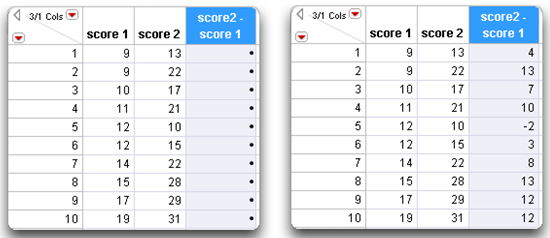
![]() Click Apply, or close the Formula Editor to see the results in the data table as shown in Figure 3.8.
Click Apply, or close the Formula Editor to see the results in the data table as shown in Figure 3.8.
Figure 3.8: Compute the Difference between Two Columns
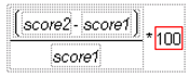
Go one step further and express the change in scores as a percentage of the base score (score1). To do this:
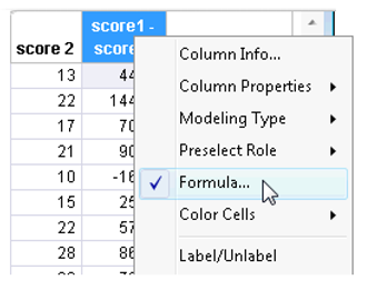
![]() Display the formula for the computed column, score2−score1. To quickly show the Formula Editor, right-click on the column header and select Formula from the menu that appears.
Display the formula for the computed column, score2−score1. To quickly show the Formula Editor, right-click on the column header and select Formula from the menu that appears.
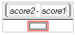
![]() The entire formula in the Formula Editor is selected. It appears enclosed in a red box. Click the divide operator (
The entire formula in the Formula Editor is selected. It appears enclosed in a red box. Click the divide operator ( ![]() ) on the keypad. The modified formula appears as a quotient with a highlighted missing denominator term.
) on the keypad. The modified formula appears as a quotient with a highlighted missing denominator term.
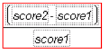
![]() Click score1 in the variable list to insert it into the denominator. Then click inside the largest box to highlight the entire formula. Alternatively, type a right parenthesis to highlight an entire formula.
Click score1 in the variable list to insert it into the denominator. Then click inside the largest box to highlight the entire formula. Alternatively, type a right parenthesis to highlight an entire formula.
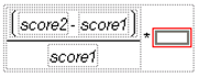
![]() Click the multiply operator (
Click the multiply operator (![]() ) on the keypad to add a term that multiplies the entire formula. The new term appears highlighted, ready to accept a value.
) on the keypad to add a term that multiplies the entire formula. The new term appears highlighted, ready to accept a value.
![]() On your keyboard, type ‘100’ to enter it as the final term. Click Apply and OK to compute the difference as a percentage of score1.
On your keyboard, type ‘100’ to enter it as the final term. Click Apply and OK to compute the difference as a percentage of score1.
![]() Finally, clean up the table. Right-click in the header area of the new computed column and select the Column Info command.
Finally, clean up the table. Right-click in the header area of the new computed column and select the Column Info command.
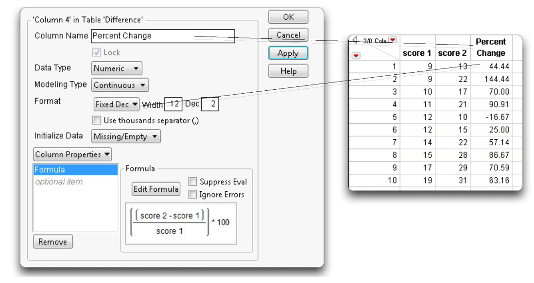
![]() In the Column Info dialog, change the column name to Percent Change. Also, select Fixed Dec from the Format menu and display the percentages with two decimal places.
In the Column Info dialog, change the column name to Percent Change. Also, select Fixed Dec from the Format menu and display the percentages with two decimal places.
Figure 3.9 shows these changes entered into the Column Info dialog and the data table.
Figure 3.9: Change Variable Name and Show Difference as a Percentage
Data Table Management
The JMP data grid holds a rectangular array of data. Rows of data usually constitute information for one subject. The columns (or variables) list information for each row. However, there are different ways to arrange the data grid, and a particular type of analysis might first require manipulating the data.
The following kinds of data rearrangement are often needed to prepare data for analysis:
- sort tables
- stack or split columns within a single table
- subset a table
- join multiple tables side by side to create a single new table
- concatenate (append) multiple tables end to end to create a single new table
The next sections explain rearranging data and include simple examples.
Sort a Table
The Sort command on the Tables menu gives standard sorting options. There is rarely a need to sort JMP tables in preparation for a statistical analysis, but you might want to view data sorted by one or more variables.
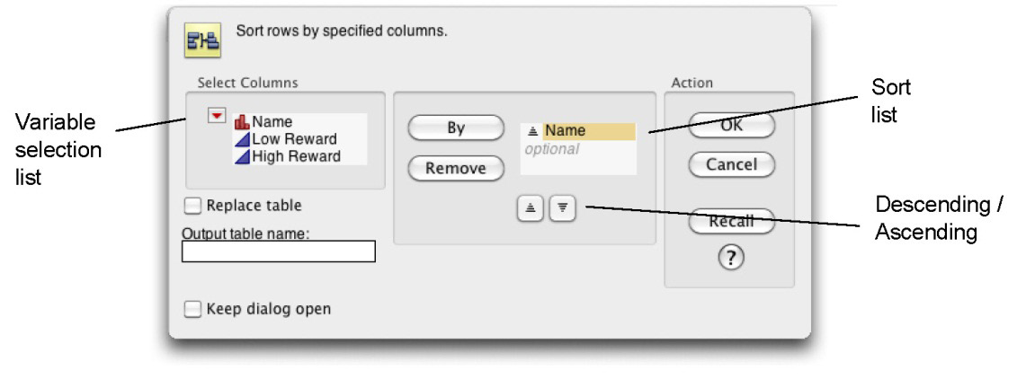
Figure 3.10 illustrates a completed Sort dialog to sort a table by a variable called Name. To sort, select one or more variables in the variable selection list, and click By to see them in the sort list. By default, the variables sort in ascending order. To sort a variable in descending order, select the variable in the sort list, and click the descending button. Note that you can sort a table in place by checking the Replace table box. If you want to preserve the original table order, enter a name in the Output table name edit box, as shown here.
Figure 3.10: Completed Sort Dialog
Stack or Split Columns
Sometimes an analysis platform looks for a specific arrangement of data, or can handle data in more than one type of arrangement. Consider the example JMP tables in Figure 3.11. These tables contain the same information arranged in different ways. Both tables have values on a commitment scale for 10 people under both low-reward and high-reward conditions.
- The table on the left splits the commitment response values into two columns called Low Reward and High Reward. The subject’s name identifies each observation.
- The table on the right stacks the commitment response values into a single column called Commitment Value. Each observation is identified by both the subject’s name and the reward condition that corresponds to the recorded commitment value.
In the chapters that follow, data tables are in the arrangement needed for examples, but you might receive data with multiple columns that you want arranged into a single column. Or, there could be values listed in a single column that you want split into multiple columns. The Tables menu has Stack and Split commands that rearrange data into a new data table.
The following steps show how to stack and split columns.
![]() Open the commitment paired.jmp table, which is shown on the left in Figure 3.11.
Open the commitment paired.jmp table, which is shown on the left in Figure 3.11.
![]() Choose Stack from the Tables menu.
Choose Stack from the Tables menu.
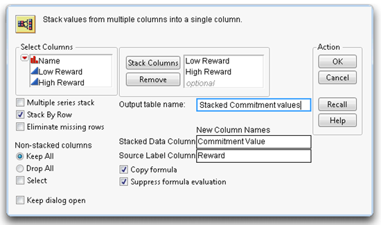
![]() Complete the Stack dialog as shown in Figure 3.12. The name of the new table is Stacked Commitment Values. If you don’t give it a name, the new table is called Untitled 1.
Complete the Stack dialog as shown in Figure 3.12. The name of the new table is Stacked Commitment Values. If you don’t give it a name, the new table is called Untitled 1.
![]() Click Stack in the Stack dialog to see the data table on the right in
Click Stack in the Stack dialog to see the data table on the right in
Figure 3.11.
The entries in the Stack dialog cause a single column to be formed by stacking the columns you add to the Stack Columns list (Low Reward and High Reward). The new column, called Commitment Value as specified in the Stack dialog, lists all the commitment scores. A new column, called Reward as seen in Figure 3.11, lists the original column name that corresponds to the response value in each row. You can stack as many columns as you want.
Figure 3.11: Split Columns (left) and Stacked Columns (right)
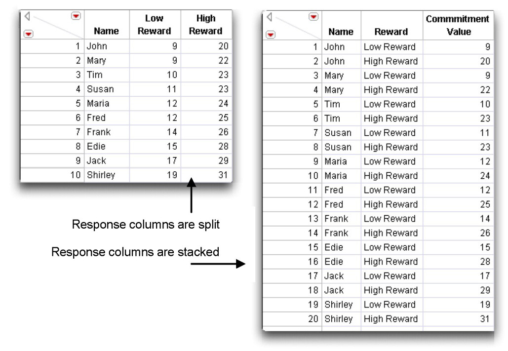
Figure 3.12: Stack Columns Dialog
Next, use the Split command to convert the stacked table (on the right in Figure 3.11) back to the original table shown on the left.
![]() With the newly created data table (Stacked Commitment Values) active, choose Split from the Tables menu.
With the newly created data table (Stacked Commitment Values) active, choose Split from the Tables menu.
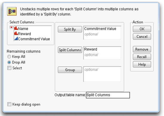
![]() Complete the Split dialog as shown in Figure 3.13. Enter Commitment Value into the Split By columns list because you want the single column of commitment scores to be split into a high reward column and a low reward column.
Complete the Split dialog as shown in Figure 3.13. Enter Commitment Value into the Split By columns list because you want the single column of commitment scores to be split into a high reward column and a low reward column.
![]() Enter Reward as the Split Columns variable. The values in the Reward column become the new column names. There are as many new (split) columns as there are values of the Split Columns variable.
Enter Reward as the Split Columns variable. The values in the Reward column become the new column names. There are as many new (split) columns as there are values of the Split Columns variable.
![]() Click the Split button. Splitting the Commitment Value column according to the values of Reward gives the original table, shown on the left in Figure 3.11.
Click the Split button. Splitting the Commitment Value column according to the values of Reward gives the original table, shown on the left in Figure 3.11.
Figure 3.13: Split Columns Dialog
Create Subsets of Data
It is not unusual to want to analyze one or more subsets of a larger data table. The most common way to create a subset from an existing table (or source table) is to use the Subset command in the Tables menu. The source table in this example is difference.jmp, which was used in the “Compute Column Values with a Formula” section.
Use the Subset Command to Create a Subset
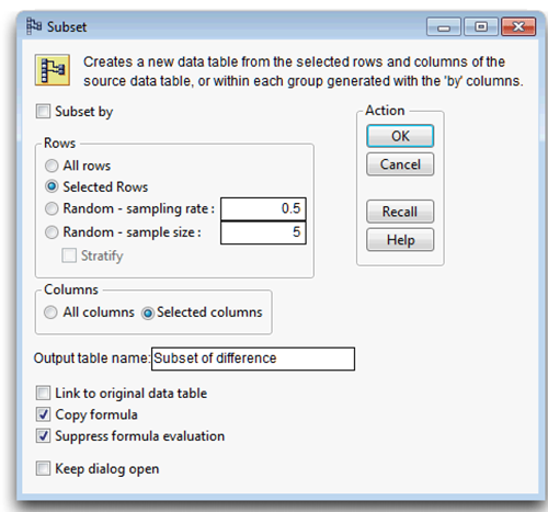
The Subset command creates a new table that consists of the highlighted rows and columns in the source table. The Subset dialog (Figure 3.14), offers these subsetting options.
- The dialog tells you to select the columns in the table to include in the new table. If no columns are selected, the new table will have all columns from the source table.
- The new table’s name displays as Subset of Source Table. You can change the name of the new table in the Subset Name text box.
- If you check the All Rows radio button, the result is a duplicate of the entire data table.
- To create a subset of just those rows you select in the source table, click the Selected Rows radio button. This is the default if any rows are selected.
- To create a random subset, click the Random Sample radio button, and enter either a decimal sample rate or the actual sample size you want.
Figure 3.14: Subset Dialog
Follow these steps to create a subset with the Subset command.
![]() Open the difference.jmp table that was used in the “ Compute Column Values with a Formula” section, and compute the percent change column as described in that section.
Open the difference.jmp table that was used in the “ Compute Column Values with a Formula” section, and compute the percent change column as described in that section.
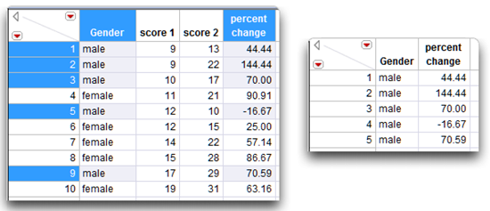
![]() Highlight the gender and the percent change columns. (Click in the column name area to highlight these columns.
Highlight the gender and the percent change columns. (Click in the column name area to highlight these columns.
![]() Highlight the rows where gender is “male.” Use control-click to highlight noncontiguous rows (option-click on the Macintosh).
Highlight the rows where gender is “male.” Use control-click to highlight noncontiguous rows (option-click on the Macintosh).
The table with highlighted rows and columns appears on the left in Figure 3.15.
Use Tables > Subset as shown before in Figure 3.14, which requests only highlighted rows and columns. Click OK to see the subset table on the right in Figure 3.15.
Figure 3.15: Subset Example
The Subset command subsets highlighted rows and columns (or all rows if none are selected, and all columns if none are selected). There are many ways to highlight rows other than manually clicking on row numbers, which is often tedious. The next section presents one simple way to create subsets using the Distribution platform.
Use a Histogram to Create a Subset
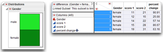
If you create a histogram and double-click on one of its bars, JMP creates a subset of the rows represented by that bar. This action highlights the corresponding rows in the analysis table, and immediately creates a subset of those rows and all selected columns (or all columns if none are selected). This ‘no frills’ subset has all formulas in the source table, as indicated by the formula icon next to percent change in Figure 3.16.
Figure 3.16: Double-Click a Histogram Bar to Create a Subset
Note: To analyze subsets of data without creating subsets, use the By option found on most analysis platforms. This option automatically analyzes data for each level of a variable (by-variable) you specify. An analysis report labeled for each by group level displays in a single window.
Concatenate Tables End to End
Research in any field often involves results from more than one group or location. The data must then be combined into a single table for analysis. In the simplest case, different tables have the same variables and you want to concatenate them—attach or append them to each other end to end.
Suppose scores for males and females are in different tables, as illustrated previously in Figure 3.15 and Figure 3.16. You can experiment with the sample files, called difference male.jmp and difference female.jmp, to see what happens when you concatenate tables.
![]() Open the difference male.jmp and the difference female.jmp data tables. Note that they have the same variables with the same names.
Open the difference male.jmp and the difference female.jmp data tables. Note that they have the same variables with the same names.
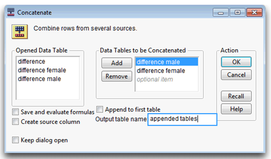
![]() Choose Concatenate from the Tables menu and complete the dialog as shown in Figure 3.17.
Choose Concatenate from the Tables menu and complete the dialog as shown in Figure 3.17.
![]() Click OK in the Concatenate dialog to see the single combined table.
Click OK in the Concatenate dialog to see the single combined table.
Figure 3.17: Concatenate Dialog
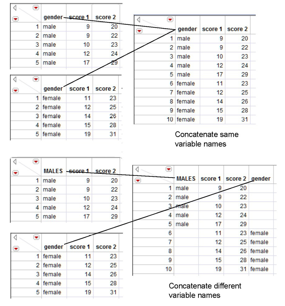
![]() Click OK in the Concatenate dialog to see the single combined table at the top in Figure 3.18.
Click OK in the Concatenate dialog to see the single combined table at the top in Figure 3.18.
In this first example the variable names are the same in the tables being concatenated. It is good to know what happens if the variables you want to concatenate have different names.
Change the variable name from gender to male in the males source tables. The tables should look like the ones at the bottom in Figure 3.18.
![]() Again choose Tables > Concatenate to combine the tables.
Again choose Tables > Concatenate to combine the tables.
Note that the concatenate action preserves all variable names. It has no way of knowing that columns with different names represent the same variable. You can correct this problem by changing the column names in the original tables to be the same and concatenating again. Or, copy the “male” values from the males column in the combined table and paste them into the empty cells of the gender column. Then use Cols > Delete Columns to eliminate the spurious males column.
Figure 3.18: Concatenate Tables with Same or Different Variable Names
Join Tables Side by Side
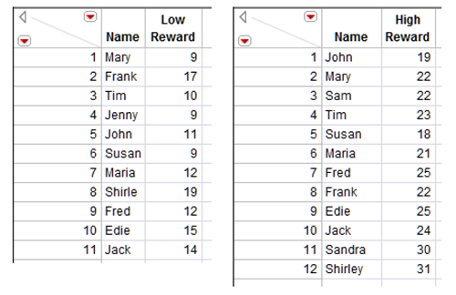
It is also not unusual to combine tables side by side, or join tables. Joining tables is necessary when different information for the same subjects is in separate tables and you want to analyze the data together. Suppose the commitment data show previously in Figure 3.11 originally existed in the two tables shown in Figure 3.19. The tables contain most of the same subjects, although the tables have different numbers of subjects. These sample data tables are called commitment low.jmp and commitment high.jmp. Note that the names are not sorted, and are not in the same order in the two tables. The JMP Join command does not require that the names be sorted in order to identify matching names in the two tables.
Figure 3.19: High Reward and Low Reward Data for the Same Subjects
The Join command in the Tables menu can combine these tables to produce the commitment paired.jmp table. Using options in the Join dialog, the combined table in this example eliminates subjects who are not in both tables.
Joining tables can be a multi-step process:
1. Identify the two tables to be joined.
2. Identify the variable(s) whose values must match for observations to be joined.
3. Select the variables to include in the new joined table.
You can see how Join works by doing this:
![]() Open the two tables called commitment high.jmp and commitment low.jmp to see the tables shown above.
Open the two tables called commitment high.jmp and commitment low.jmp to see the tables shown above.
![]() With the commitment high.jmp table active, choose Join from the Tables menu.
With the commitment high.jmp table active, choose Join from the Tables menu.
![]() Click commitment low in the selection list on the left of the dialog. Note in Figure 3.19 that commitment high displays as the join table in the initial dialog, and commitment low displays as the with table in this initial dialog.
Click commitment low in the selection list on the left of the dialog. Note in Figure 3.19 that commitment high displays as the join table in the initial dialog, and commitment low displays as the with table in this initial dialog.
The Matching Specification radio buttons let you choose from three kinds of join.
- By Row Number combines the first row in the join table with the first row in the with table, the second rows in each table, and so on. No consideration is given to the values of any variables.
- Cartesian Join combines each row in the join table with each row in the with table. This can produce a large table if there are many observations in the tables to be joined. The total number of observations in the Cartesian joined table is the number of rows in the join table multiplied by the number of rows in the with table.
- By Matching Columns combines rows from each table only if the values of the columns you specify are the same.
Because the data tables in this example contain information for the same subjects, identified by name, you want to match the observations by name. That is, observations should only be joined when the names match.
![]() Click the By Matching Columns radio button in the Join dialog.
Click the By Matching Columns radio button in the Join dialog.
![]() Select Name in the box for each table showing at the lower left of the dialog, and click Match. The variables to be matched appear in the Match columns panel as shown in Figure 3.20. You can have as many match variables as you need.
Select Name in the box for each table showing at the lower left of the dialog, and click Match. The variables to be matched appear in the Match columns panel as shown in Figure 3.20. You can have as many match variables as you need.
Note that the checkboxes at the bottom of the Match Columns dialog are not checked. In particular, by leaving the Include Non Matches unchecked, only those observations that occur in both tables are included in the new joined table.
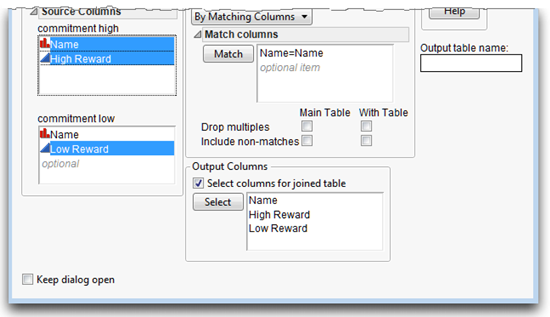
If you finish the join now, all variables from both tables appear in the new joined table, but it isn’t necessary to include the matching variable (Name) from both tables. To include Name only once,
![]() Click the Select columns for joined table box in the Join dialog.
Click the Select columns for joined table box in the Join dialog.
![]() Complete the Select Columns dialog as shown in Figure 3.21.
Complete the Select Columns dialog as shown in Figure 3.21.
Now you are ready to complete the join. Optionally, enter a name for the new joined table in the Output Table text box.
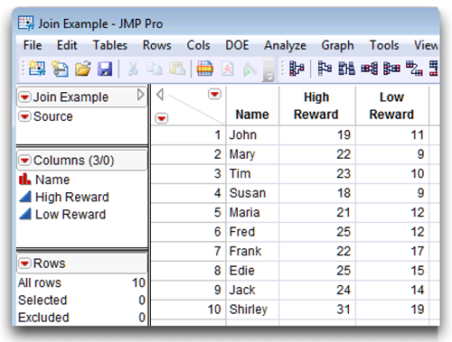
![]() Click OK in the Join dialog to see the table in Figure 3.22.
Click OK in the Join dialog to see the table in Figure 3.22.
Figure 3.20: Join Dialog for Matched Join
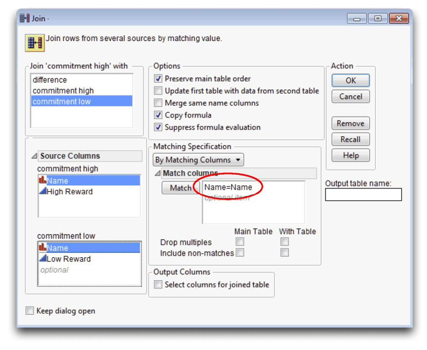
Figure 3.21: Select Columns for Join
The final joined table has the 10 observations that had matching values. The observations are in the order found in the first table listed on the Join dialog.
Figure 3.22: Table Created by Joining Two Tables
Summary
All computer programs that do statistical analyses require that data be in a form recognized by the program. Although most tables used as examples can be found on the author page for this book, your own data must be entered or read into a JMP data table. This chapter presented an overview of JMP data tables, including
- the structure and form of a JMP data table
- how to create and delete rows and columns
- how to get data into a JMP table
- how to compute column values
- how to stack and split columns in a data table
- how to create subsets of data
- how to combine tables side by side (join) and end to end (concatenate)
The information presented is designed to get you started. Details and extensive examples can be found in Using JMP (2012). This book and all the JMP books are available on the Help menu.
References
SAS Institute Inc. 2012. Using JMP. Cary, NC: SAS Institute Inc.