Chapter 5. Learning multiple weights at a time: generalizing gradient descent

In this chapter

• Gradient descent learning with multiple inputs
• Freezing one weight: what does it do?
• Gradient descent learning with multiple outputs
• Gradient descent learning with multiple inputs and outputs
• Visualizing weight values
• Visualizing dot products

“You don’t learn to walk by following rules. You learn by doing and by falling over.”

Richard Branson, http://mng.bz/oVgd

Gradient descent learning with multiple inputs

Gradient descent also works with multiple inputs

In the preceding chapter, you learned how to use gradient descent to update a weight. In this chapter, we’ll more or less reveal how the same techniques can be used to update a network that contains multiple weights. Let’s start by jumping in the deep end, shall we? The following diagram shows how a network with multiple inputs can learn.

There’s nothing new in this diagram. Each weight_delta is calculated by taking its output delta and multiplying it by its input. In this case, because the three weights share the same output node, they also share that node’s delta. But the weights have different weight deltas owing to their different input values. Notice further that you can reuse the ele_mul function from before, because you’re multiplying each value in weights by the same value delta.

Gradient descent with multiple inputs explained

Simple to execute, and fascinating to understand

When put side by side with the single-weight neural network, gradient descent with multiple inputs seems rather obvious in practice. But the properties involved are fascinating and worthy of discussion. First, let’s take a look at them side by side.

Up until the generation of delta on the output node, single input and multi-input gradient descent are identical (other than the prediction differences we studied in chapter 3). You make a prediction and calculate error and delta in identical ways. But the following problem remains: when you had only one weight, you had only one input (one weight_delta to generate). Now you have three. How do you generate three weight_deltas?

How do you turn a single delta (on the node) into three weight_delta values?

Remember the definition and purpose of delta versus weight_delta. delta is a measure of how much you want a node’s value to be different. In this case, you compute it by a direct subtraction between the node’s value and what you wanted the node’s value to be (pred - true). Positive delta indicates the node’s value was too high, and negative that it was too low.

weight_delta, on the other hand, is an estimate of the direction and amount to move the weights to reduce node_delta, inferred by the derivative. How do you transform delta into a weight_delta? You multiply delta by a weight’s input.

Consider this from the perspective of a single weight, highlighted at right:

• delta: Hey, inputs—yeah, you three. Next time, predict a little higher.
• Single weight: Hmm: if my input was 0, then my weight wouldn’t have mattered, and I wouldn’t change a thing (stopping). If my input was negative, then I’d want to decrease my weight instead of increase it (negative reversal). But my input is positive and quite large, so I’m guessing that my personal prediction mattered a lot to the aggregated output. I’m going to move my weight up a lot to compensate (scaling).

The single weight increases its value.

What did those three properties/statements really say? They all (stopping, negative reversal, and scaling) made an observation of how the weight’s role in delta was affected by its input. Thus, each weight_delta is a sort of input-modified version of delta.

This brings us back to the original question: how do you turn one (node) delta into three weight_delta values? Well, because each weight has a unique input and a shared delta, you use each respective weight’s input multiplied by delta to create each respective weight_delta. Let’s see this process in action.

In the next two figures, you can see the generation of weight_delta variables for the previous single-input architecture and for the new multi-input architecture. Perhaps the easiest way to see how similar they are is to read the pseudocode at the bottom of each figure. Notice that the multi-weight version multiplies delta (0.14) by every input to create the various weight_deltas. It’s a simple process.

The last step is also nearly identical to the single-input network. Once you have the weight_delta values, you multiply them by alpha and subtract them from the weights. It’s literally the same process as before, repeated across multiple weights instead of a single one.

Let’s watch several steps of learning

def neural_network(input, weights):
  out = 0
  for i in range(len(input)):
    out += (input[i] * weights[i])
  return out

def ele_mul(scalar, vector):
  out = [0,0,0]
  for i in range(len(out)):
    out[i] = vector[i] * scalar
  return out

toes = [8.5, 9.5, 9.9, 9.0]
wlrec = [0.65, 0.8, 0.8, 0.9]
nfans = [1.2, 1.3, 0.5, 1.0]

win_or_lose_binary = [1, 1, 0, 1]
true = win_or_lose_binary[0]

alpha = 0.01
weights = [0.1, 0.2, -.1]
input = [toes[0],wlrec[0],nfans[0]]

for iter in range(3):

  pred = neural_network(input,weights)

  error = (pred - true) ** 2
  delta = pred - true

  weight_deltas=ele_mul(delta,input)

  print("Iteration:" + str(iter+1))
  print("Pred:" + str(pred))
  print("Error:" + str(error))
  print("Delta:" + str(delta))
  print("Weights:" + str(weights))
  print("Weight_Deltas:")
  print(str(weight_deltas))
  print(
  )

  for i in range(len(weights)):
    weights[i]-=alpha*weight_deltas[i]

We can make three individual error/weight curves, one for each weight. As before, the slopes of these curves (the dotted lines) are reflected by the weight_delta values. Notice that a is steeper than the others. Why is weight_delta steeper for a than the others if they share the same output delta and error measure? Because a has an input value that’s significantly higher than the others and thus, a higher derivative.

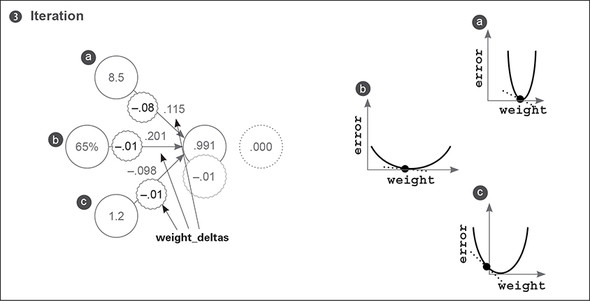
Here are a few additional takeaways. Most of the learning (weight changing) was performed on the weight with the largest input a, because the input changes the slope significantly. This isn’t necessarily advantageous in all settings. A subfield called normalization helps encourage learning across all weights despite dataset characteristics such as this. This significant difference in slope forced me to set alpha lower than I wanted (0.01 instead of 0.1). Try setting alpha to 0.1: do you see how a causes it to diverge?

Freezing one weight: What does it do?

This experiment is a bit advanced in terms of theory, but I think it’s a great exercise to understand how the weights affect each other. You’re going to train again, except weight a won’t ever be adjusted. You’ll try to learn the training example using only weights b and c (weights[1] and weights[2]).

def neural_network(input, weights):
  out = 0
  for i in range(len(input)):
    out += (input[i] * weights[i])
  return out

def ele_mul(scalar, vector):
  out = [0,0,0]
  for i in range(len(out)):
    out[i] = vector[i] * scalar
  return out

toes = [8.5, 9.5, 9.9, 9.0]
wlrec = [0.65, 0.8, 0.8, 0.9]
nfans = [1.2, 1.3, 0.5, 1.0]

win_or_lose_binary = [1, 1, 0, 1]
true = win_or_lose_binary[0]

alpha = 0.3
weights = [0.1, 0.2, -.1]
input = [toes[0],wlrec[0],nfans[0]]

for iter in range(3):
  pred = neural_network(input,weights)

  error = (pred - true) ** 2
  delta = pred - true

  weight_deltas=ele_mul(delta,input)
  weight_deltas[0] = 0

  print("Iteration:" + str(iter+1))
  print("Pred:" + str(pred))
  print("Error:" + str(error))
  print("Delta:" + str(delta))
  print("Weights:" + str(weights))
  print("Weight_Deltas:")
  print(str(weight_deltas))
  print(
  )

  for i in range(len(weights)):
    weights[i]-=alpha*weight_deltas[i]

Perhaps you’re surprised to see that a still finds the bottom of the bowl. Why is this? Well, the curves are a measure of each individual weight relative to the global error. Thus, because error is shared, when one weight finds the bottom of the bowl, all the weights find the bottom of the bowl.

This is an extremely important lesson. First, if you converged (reached error = 0) with b and c weights and then tried to train a, a wouldn’t move. Why? error = 0, which means weight_delta is 0. This reveals a potentially damaging property of neural networks: a may be a powerful input with lots of predictive power, but if the network accidentally figures out how to predict accurately on the training data without it, then it will never learn to incorporate a into its prediction.

Also notice how a finds the bottom of the bowl. Instead of the black dot moving, the curve seems to move to the left. What does this mean? The black dot can move horizontally only if the weight is updated. Because the weight for a is frozen for this experiment, the dot must stay fixed. But error clearly goes to 0.

This tells you what the graphs really are. In truth, these are 2D slices of a four-dimensional shape. Three of the dimensions are the weight values, and the fourth dimension is the error. This shape is called the error plane, and, believe it or not, its curvature is determined by the training data. Why is that the case?

error is determined by the training data. Any network can have any weight value, but the value of error given any particular weight configuration is 100% determined by data. You’ve already seen how the steepness of the U shape is affected by the input data (on several occasions). What you’re really trying to do with the neural network is find the lowest point on this big error plane, where the lowest point refers to the lowest error. Interesting, eh? We’ll come back to this idea later, so file it away for now.

Gradient descent learning with multiple outputs

Neural networks can also make multiple predictions using only a single input

Perhaps this will seem a bit obvious. You calculate each delta the same way and then multiply them all by the same, single input. This becomes each weight’s weight_delta. At this point, I hope it’s clear that a simple mechanism (stochastic gradient descent) is consistently used to perform learning across a wide variety of architectures.

 

Gradient descent with multiple inputs and outputs

Gradient descent generalizes to arbitrarily large networks

 

What do these weights learn?

Each weight tries to reduce the error, but what do they learn in aggregate?

Congratulations! This is the part of the book where we move on to the first real-world dataset. As luck would have it, it’s one with historical significance.

It’s called the Modified National Institute of Standards and Technology (MNIST) dataset, and it consists of digits that high school students and employees of the US Census Bureau handwrote some years ago. The interesting bit is that these handwritten digits are black-and-white images of people’s handwriting. Accompanying each digit image is the actual number they were writing (0–9). For the last few decades, people have been using this dataset to train neural networks to read human handwriting, and today, you’re going to do the same.

Each image is only 784 pixels (28 × 28). Given that you have 784 pixels as input and 10 possible labels as output, you can imagine the shape of the neural network: each training example contains 784 values (one for each pixel), so the neural network must have 784 input values. Pretty simple, eh? You adjust the number of input nodes to reflect how many datapoints are in each training example. You want to predict 10 probabilities: one for each digit. Given an input drawing, the neural network will produce these 10 probabilities, telling you which digit is most likely to be what was drawn.

How do you configure the neural network to produce 10 probabilities? In the previous section, you saw a diagram for a neural network that could take multiple inputs at a time and make multiple predictions based on that input. You should be able to modify this network to have the correct number of inputs and outputs for the new MNIST task. You’ll tweak it to have 784 inputs and 10 outputs.

In the MNISTPreprocessor notebook is a script to preprocess the MNIST dataset and load the first 1,000 images and labels into two NumPy matrices called images and labels. You may be wondering, “Images are two-dimensional. How do I load the (28 × 28) pixels into a flat neural network?” For now, the answer is simple: flatten the images into a vector of 1 × 784. You’ll take the first row of pixels and concatenate them with the second row, and the third row, and so on, until you have one list of pixels per image (784 pixels long).

This diagram represents the new MNIST classification neural network. It most closely resembles the network you trained with multiple inputs and outputs earlier. The only difference is the number of inputs and outputs, which has increased substantially. This network has 784 inputs (one for each pixel in a 28 × 28 image) and 10 outputs (one for each possible digit in the image).

If this network could predict perfectly, it would take in an image’s pixels (say, a 2, like the one in the next figure) and predict a 1.0 in the correct output position (the third one) and a 0 everywhere else. If it were able to do this correctly for all the images in the dataset, it would have no error.

Over the course of training, the network will adjust the weights between the input and prediction nodes so that error falls toward 0 in training. But what does this do? What does it mean to modify a bunch of weights to learn a pattern in aggregate?

Visualizing weight values

An interesting and intuitive practice in neural network research (particularly for image classifiers) is to visualize the weights as if they were an image. If you look at this diagram, you’ll see why.

Each output node has a weight coming from every pixel. For example, the 2? node has 784 input weights, each mapping the relationship between a pixel and the number 2.

What is this relationship? Well, if the weight is high, it means the model believes there’s a high degree of correlation between that pixel and the number 2. If the number is very low (negative), then the network believes there is a very low correlation (perhaps even negative correlation) between that pixel and the number 2.

If you take the weights and print them out into an image that’s the same shape as the input dataset images, you can see which pixels have the highest correlation with a particular output node. In our example, a very vague 2 and 1 appear in the two images, which were created using the weights for 2 and 1, respectively. The bright areas are high weights, and the dark areas are negative weights. The neutral color (red, if you’re reading this in the eBook) represents 0 in the weight matrix. This illustrates that the network generally knows the shape of a 2 and of a 1.

Why does it turn out this way? This takes us back to the lesson on dot products. Let’s have a quick review.

Visualizing dot products (weighted sums)

Recall how dot products work. They take two vectors, multiply them together (elementwise), and then sum over the output. Consider this example:

a = [ 0, 1, 0, 1]
b = [ 1, 0, 1, 0]

    [ 0, 0, 0, 0] -> 0    1

• 1 Score

First you multiply each element in a and b by each other, in this case creating a vector of 0s. The sum of this vector is also 0. Why? Because the vectors have nothing in common.

c = [ 0, 1, 1, 0]            b = [ 1, 0, 1, 0]
d = [.5, 0,.5, 0]            c = [ 0, 1, 1, 0]

But the dot products between c and d return higher scores, because there’s overlap in the columns that have positive values. Performing dot products between two identical vectors tends to result in higher scores, as well. The takeaway? A dot product is a loose measurement of similarity between two vectors.

What does this mean for the weights and inputs? Well, if the weight vector is similar to the input vector for 2, then it will output a high score because the two vectors are similar. Inversely, if the weight vector is not similar to the input vector for 2, it will output a low score. You can see this in action in the following figure. Why is the top score (0.98) higher than the lower one (0.01)?

Summary

Gradient descent is a general learning algorithm

Perhaps the most important subtext of this chapter is that gradient descent is a very flexible learning algorithm. If you combine weights in a way that allows you to calculate an error function and a delta, gradient descent can show you how to move the weights to reduce the error. We’ll spend the rest of this book exploring different types of weight combinations and error functions for which gradient descent is useful. The next chapter is no exception.