- Defining and playing sound waves with Python and PyGame
- Turning sinusoidal functions into playable musical notes
- Combining two sounds by adding their sound waves as functions
- Decomposing a sound wave function into its Fourier series to see its musical notes
For a lot of part 2, we’ve focused on using calculus to simulate moving objects. In this chapter, I’ll show you a completely different application: working with audio data. Digital audio data is a computer representation of sound waves, which are repeating changes of pressure in the air that our ears perceive as sound. We’ll think of sound waves as functions that we can add and scale as vectors, and then we can use integrals to understand what kinds of sounds they represent. As a result, our exploration of sound waves combines a lot of what you’ve learned about both linear algebra and calculus in earlier chapters.
I won’t go too deep into the physics of sound waves, but it’s useful to understand how they work at a basic level. What we perceive as sound isn’t air pressure itself, but rather rapid changes in air pressure that cause our eardrums to vibrate. For instance, if you play a violin, you drag the bow across one of the strings and cause the string to vibrate. The vibrating string causes the air around it to rapidly change pressure, and the changes in pressure propagate through the air as sound waves until they reach your ear. At that point, your eardrum vibrates at the same rate, and you perceive a sound (figure 13.1).

Figure 13.1 Schematic diagram of the sound of a violin reaching an eardrum
You can think of a digital audio file as a function describing a vibration over time. Audio software interprets the function and instructs your speakers to vibrate accordingly, producing sound waves of a similar shape in the air around the speakers. For our purposes, it doesn’t matter exactly what the function represents, but you can interpret it loosely as describing air pressure over time (figure 13.2).

Figure 13.2 Thinking of sound waves as functions, loosely interpreted as representing pressure over time
Interesting sounds like musical notes have sound waves with repeating patterns, like the one shown in figure 13.2. The rate at which the function repeats itself is called the frequency and tells how high or low the musical note sounds. The quality, or timbre, of the sound is controlled by the shape of the repeating pattern, for instance, whether it sounds more like a violin, a trumpet, or a human voice.
13.1 Combining sound waves and decomposing them
Throughout this chapter, we do mathematical operations on functions and use Python to play them as actual sounds. The two main things we’ll do are combining existing sound waves to make new ones and then decomposing complex sound waves into simpler ones. For instance, we can combine several musical notes into a chord and then we can decompose a chord to see its musical notes.
Before we do that, however, we need to cover the basic building blocks: sound waves and musical notes. I start by showing you how to use Python to turn a sequence of numbers, representing a sound wave, into a real sound coming out of your speakers. To make a sound corresponding to a function, we extract some y values from the graph of the function and pass these to the audio library as an array. This is a process called sampling(figure 13.3).
The main sound wave functions we’ll use are periodic functions, whose graphs are built from the same repeating shape. Specifically, we’ll use sinusoidal functions, a family of periodic functions including sine and cosine that produce natural-sounding musical notes. After sampling them to turn them into sequences of numbers, we’ll build Python functions to play musical notes.
Once we can produce individual notes, we’ll write Python code to help us combine different notes to create chords and other complex sounds. We’ll do this by adding the functions defining each of the sound waves together. We’ll see that combining a few musical notes can make a chord, and combining dozens of musical notes together can produce some quite interesting and qualitatively dissimilar sounds.

Figure 13.3 Starting with the graph of a function f(t) (top) and sampling some of the y values (bottom) to send to an audio library
Our last goal will be to decompose a function representing any sound wave into a sum of (pure) musical notes and their corresponding volumes, which make up the sound wave (figure 13.4). Such a decomposition into a sum is called a Fourier series(pronounced FOR-ee-yay). Once we’ve found the sound waves making up a Fourier series, we can play them together and get the original sound.

Figure 13.4 Decomposing a sound wave function into a combination of simpler ones using a Fourier series
Mathematically, finding a Fourier series means writing a function as a sum or, more specifically, a linear combination of sine and cosine functions. This procedure and its variants are among the most important algorithms of all time. Methods similar to the ones we’ll cover are used in common applications like MP3 compression, as well as in more grandiose ones like the recent Nobel prize-winning detection of gravitational waves.
It’s one thing to look at these sound waves as graphs, but it’s another to actually hear them coming out of your speakers. Let’s make some noise!
13.2 Playing sound waves in Python
To play sounds in Python, we turn to the PyGame library that we used in a few of the preceding chapters. A particular function in this library takes an array of numbers as input and plays a sound as a result. As a first step, we use a random sequence of numbers in Python and write code to interpret and play these sounds with PyGame. This will just be noise(yes, that’s a technical term!) rather than beautiful music at this point, but we need to start somewhere.
After producing some noise, we’ll make a slightly more appealing sound by running the same process on a sequence of numbers that have repeating patterns, rather than just being completely random. This sets us up for the next section, where we’ll get a sequence of repeating numbers by sampling a periodic function.
13.2.1 Producing our first sound
Before we pass PyGame an array of numbers representing a sound, we need to tell it how the numbers should be interpreted. There are several technical details about audio data here, and I’ll explain them so you know how PyGame thinks about that, but these details won’t be critical to the rest of the chapter.
In this application, we use conventions typically used in CD audio. Specifically, we’ll represent one second of audio with an array of 44,100 values, each of which is a 16-bit integer (between −32,768 and 32,767). These numbers roughly represent the intensity of the sound at every step of time, with 44,100 steps in a second. This is not unlike how we represented an image in chapter 6. Instead of an array of values giving the brightness of pixels, we have an array of values giving the intensity of a sound wave at different moments in time. Eventually, we’ll get these numbers as the y-coordinates of points on a sound wave graph, but for now, we’re going to pick them randomly to make some noise.
We also use a single channel, meaning we only play one sound wave as opposed to stereo audio, which produces two sound waves simultaneously, one in the left speaker and one in the right. The other thing we configure is the bit depth of the sound. While frequency is analogous to the resolution of an image, bit depth is like the number of allowable pixel colors, more bit depth means a more refined range of sound intensities. We used three numbers between 0 and 256 for the color of a pixel, but here, we use a single 16-bit number to represent the sound intensity at a moment in time. With these parameters selected, the first step in our code is to import PyGame and initialize the sound library:
>>> import pygame, pygame.sndarray
>>> pygame.mixer.init(frequency=44100,
                      size=−16,          ❶
                      channels=1)
❶ −16 indicates a bit depth of 16 and an input of 16-bit signed integers ranging from −32,768 to 32,767
To start with the simplest possible example, we can generate one second of audio by creating a NumPy array of 44,100 random integers between −32,768 and 32,767. We can do this in one line with NumPy’s randint function:
>>> import numpy as np
>>> arr = np.random.randint(−32768, 32767, size=44100)
>>> arr
array([−16280, 30700, −12229, ..., 2134, 11403, 13338])
To interpret this array as a sound wave, we can plot its first few values on a scatter graph. I’ve included a plot_sequence function in the source code for this book to help you quickly plot an array of integer values like this. If you run plot_sequence (arr,max=100), you get a picture of the first 100 values of this array. As compared to numbers sampled from a smooth function, these numbers are all over the place (figure 13.5).

Figure 13.5 Sampled values from a sound wave (left) vs. our random values (right)
If you connect the dots, you can picture them as defining a function over this time period. Figure 13.6 shows two graphs of the array of numbers with the dots connected, showing the first 100 and 441 numbers, respectively. This data is completely random, so there’s nothing particularly interesting to see, but this will be the first sound wave we play.
Because 44,100 values define the whole second of sound, the 441 values on the bottom define the sound during the first one-hundredth of a second. Next, we can play the sound using a library call.

Figure 13.6 The first 100 values (top) and the first 441 values (bottom) connected to define a function
CAUTION Before you run the next few lines of Python code, make sure your speaker volume isn’t too high. The first sound we’ve made won’t be that pleasant, not to mention, you don’t want to hurt your ears!
To play the sound, you can run:
sound = pygame.sndarray.make_sound(arr)
sound.play()
The result should sound like one second of static, as if you turned on the radio without tuning it to a station. A sound wave like this, consisting of random values over time, is called white noise.
About the only thing you can adjust about white noise is the volume. The human ear responds to changes in pressure, and the bigger the sound wave, the bigger the changes in pressure, and the louder the perceived sound. If this white noise was unpleasantly loud for you, you can create a quieter version by generating sound data consisting of smaller numbers. For instance, this white noise is generated by numbers ranging from −10,000 to 10,000:
arr = np.random.randint(−10000, 10000, size=44100)
sound = pygame.sndarray.make_sound(arr)
sound.play()
This sound should be nearly identical to the first white noise you played, except that it is quieter. The loudness of a sound wave depends on how big the function values are, and the measure of this is called the amplitude of the wave. In this case, because the values vary 10,000 units from the average value of 0, the amplitude is said to be 10,000.
Although some people find white noise soothing, it’s not very interesting. Let’s produce a more interesting sound, namely a musical note.
13.2.2 Playing a musical note
When we hear a musical note, our ears are detecting a pattern in the vibrations in contrast to the randomness of white noise. We can put together a series of 44,100 numbers with an obvious pattern, and you’ll hear them produce a musical note. Specifically, let’s start by repeating the number 10,000 fifty times and then repeating the number −10,000 fifty times. I picked 10,000 because we just saw it’s a big enough amplitude to make the sound wave audible. Figure 13.7 shows the plot for the first 100 numbers returned from the following code snippet:
form = np.repeat([10000,−10000],50)     ❶
plot_sequence(form)
❶ Repeats each value in the list the specified number of times
If we repeat this sequence of 100 numbers 441 times, we have 44,100 total values that define one second of audio. To achieve this, we can use another handy NumPy function, called tile, which repeats a given array a specified number of times:
arr = np.tile(form,441)

Figure 13.7 A plot of the sequence, consisting of the number 10,000 repeated 50 times followed by the number −10,000 repeated 50 times.
Figure 13.8 shows the plot of the first 1,000 values of the array with the “dots” connected. You can see that it jumps back and forth between 10,000 and −10,000 every 50 numbers. That means the pattern repeats every 100 numbers.

Figure 13.8 A plot of the first 1,000 of 44,100 numbers shows the repeating pattern.
This waveform is called a square wave because its graph has sharp, 90° corners. (Note that the vertical lines are only there because MatPlotLib connects all of the dots; there are no values of the sequence between 10,000 and −10,000, just a dot at 10,000 connected to a dot at −10,000.)
The 44,100 numbers represent one second, so the 1,000 numbers graphed in figure 13.8 represent 1/44.1 seconds (or 0.023 seconds) of audio. Playing this sound data using the following lines produces a clear musical note. This is approximately the note A (or A4 in scientific pitch notation). You can listen to it with the same play() method as used in section 13.2.1:
sound = pygame.sndarray.make_sound(arr)
sound.play()
The rate of repetition (in this case, 441 repetitions per second) is called the frequency of the sound wave, and it determines the pitch of the note, or how high or low the note sounds. Frequencies of repetition are measured in units of hertz, abbreviated Hz, where 441 Hz means the same thing as 441 per second. The most common definition for the pitch A is 440 Hz, but 441 is close enough, and it conveniently divides the CD sampling rate of 44,100 values per second.
Interesting sound waves come from periodic functions, which repeat themselves on fixed intervals like the square wave in figure 13.8. The repeated sequence for the square wave consists of 100 numbers, and we repeat it 441 times to get 44,100 numbers giving one second of audio. That’s a repetition rate of 441 Hz or once every 0.0023 seconds. What our ear detects as a musical note is this rate of repetition. In the next section, we’ll play sounds corresponding to the most important periodic functions, sine and cosine, at different frequencies.
13.2.3 Exercises
form = np.repeat([10000,−10000],63) arr = np.tile(form,350) sound = pygame.sndarray.make_sound(arr) sound.play() |
13.3 Turning a sinusoidal wave into a sound
The sound we played with the square wave was a recognizable musical note, but it wasn’t very natural sounding. That’s because in nature, things don’t usually vibrate in square waves. More often, vibrations are sinusoidal, meaning if we measure and graph these, we get results that look like the graphs of the sine or cosine functions. These functions turn out to be mathematically natural as well, so we can use them as the building blocks for the music we’re going to make. After sampling the notes and passing them to PyGame, you’ll be able to hear the difference between a square wave and a sinusoidal wave.
13.3.1 Making audio from sinusoidal functions
The sinusoidal functions sine and cosine, which we’ve used several times already in this book, are intrinsically periodic functions. That’s because their inputs are interpreted as angles; if you rotate 360° or 2π radians, you’re back where you started, and the sine and cosine functions return the same values. Therefore, sin(t) and cos(t) repeat themselves every 2π units as shown in figure 13.9.

Figure 13.9 Every 2π units, the function sin(t) repeats the same value.
This interval of repetition is called the period of the periodic function, so for both sine and cosine, the period is 2π. When you graph them (figure 13.10), you can see that they look the same between 0 and 2π as they do between 2π and 4π, or between 4π and 6π, and so on.

Figure 13.10 Because the sine function is periodic with period 2π, its graph has the same shape over every 2π interval.
The only difference for the cosine function is that the graph is shifted by π/2 units to the left, but it still repeats itself every 2π units (figure 13.11).

Figure 13.11 The graph of the cosine function has the same shape as the graph of the sine function, but it is shifted to the left. It also repeats itself every 2π units.
For the purposes of audio, one repetition every 2π seconds is a frequency of 1/2π or about 0.159 Hz, which turns out to be too small to be audible by the human ear. The amplitude of 1.0 also turns out to be too small to hear in 16-bit audio. To solve this, let’s write a Python function, make_sinusoid(frequency,amplitude), which produces a sine function that is stretched or compressed vertically and horizontally to have a more desirable frequency and amplitude. A frequency of 441 Hz and an amplitude of 10,000 should represent an audible sound wave.
Once we’ve produced that function, we want to extract 44,100 evenly spaced values of the function to pass to PyGame. The process of extracting function values like this is called sampling, so we can write a function called sample(f,start,end,count) that gets the specified count number of values of f(t) in the range of t values between start and end. Once we have our desired sinusoid function, we can run sample (sinusoid,0,1,44100) to get an array of 44,100 samples to pass to PyGame, and we’ll hear what a sinusoidal wave sounds like.
13.3.2 Changing the frequency of a sinusoid
As a first example, let’s create a sinusoid with a frequency of 2, meaning a function shaped like a sine graph but repeating itself twice between zero and one. The period of the sine function is 2π, so by default, it takes 4π units to repeat itself twice (figure 13.12).
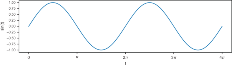
Figure 13.12 The sine function repeats itself twice between t = 0 and t = 4π.
To get two periods of the sine function graph, we need the sine function to receive values from 0 to 4π as inputs, but we want the input variable t to vary from 0 to 1. To achieve that, we can use the function sin(4πt). From t = 0 to t = 1, all of the values between 0 and 4π are passed to the sine function. The plot of sin(4πt) in figure 13.13 has the same graph as figure 13.12 but with two full periods of the sine function squished into the first 1.0 units.

Figure 13.13 The graph of sin(4πt) is sinusoidal, repeating itself twice in every unit of t for a frequency of 2.
The period of the function sin(4πt) is ½ instead of 2π, so the “squishing factor” is 4π. That is, the original period was 2π, and the reduced period is 4π times shorter. In general, for any constant k, a function of the form f(t) = sin(kt) has a period shrunk by a factor of k to 2π/ k. The frequency is increased by a factor of k from the usual value of 1/(2π) to k/2π.
If we want a sinusoidal function with a frequency of 441, the appropriate value of k would be 441 · 2 · π. That gives us a frequency of

Increasing the amplitude of the sinusoid is simpler by comparison. All you need to do is multiply the sine function by a constant factor, and the amplitude increases by the same factor. With that, we have what we need to define our make_sinusoid function:
def make_sinusoid(frequency,amplitude):
    def f(t):                                      ❶
        return amplitude * sin(2*pi*frequency*t)   ❷
    return f
❶ Defines f(t)−the sinusoidal function that is returned
❷ Multiplies the input t by 2 ⋅ π times the frequency, then multiplies the output of the sine function by the amplitude
We can test this, for example, by making a sinusoidal function with a frequency of 5 and an amplitude of 4, and plotting it (figure 13.14) from t = 0 to t = 1:
>>> plot_function(make_sinusoid(5,4),0,1)

Figure 13.14 The graph of make_sinusoid(5,4) has a height (amplitude) of 4 and repeats itself 5 times from t = 0 to t = 5, so it has a frequency of 5.
Next, we work with the sound wave function that is the result of make_sinusoid (441,8000) having a frequency of 441 Hz and an mplitude of 8,000.
13.3.3 Sampling and playing the sound wave
To play the sound wave mentioned in the last section, we need to sample it to get the array of numbers that are playable by PyGame. Let’s set
sinusoid = make_sinusoid(441,8000)
so the sinusoid function from t = 0 to t = 1 represents 1 second of a sound wave we try to play. We pick 44,100 values of t, evenly spaced between 0 and 1, and the resulting function values are the corresponding values of sinusoid(t).
We can use the NumPy function np.arange, which provides evenly spaced numbers on a given interval. For instance, np.arange(0,1,0.1) gives 10 evenly spaced values, starting from 0 and below 1 at 0.1 unit intervals:
>>> np.arange(0,1,0.1)
array([0. , 0.1, 0.2, 0.3, 0.4, 0.5, 0.6, 0.7, 0.8, 0.9])
For our application, we want to use 44,100 time values between 0 and 1, which are evenly spaced by 1/44100 units:
>>> np.arange(0,1,1/44100)
array([0.00000000e+00, 2.26757370e-05, 4.53514739e-05, ...,
       9.99931973e-01, 9.99954649e-01, 9.99977324e-01])
We want to apply the sinusoid function to every entry of this array to produce another NumPy array as a result. The NumPy function np.vectorize(f) takes a Python function f and produces a new one that applies the same operation to every entry of an array. So for us, np.vectorize(sinusoid)(arr) applies the sinusoid function to every entry of an array.
This is almost a complete procedure for sampling a function. The last detail we need to include is converting the outputs to 16-bit integer values using the astype method on NumPy arrays. Putting these steps together, we can build the following general sampling function:
def sample(f,start,end,count):                    ❶
    mapf = np.vectorize(f)                        ❷
    ts = np.arange(start,end,(end-start)/count)   ❸
    values = mapf(ts)                             ❹
    return values.astype(np.int16)                ❺
❶ Inputs are the function f to sample the start and end of the range and the number of values we want.
❷ Creates a version of f that can be applied to a NumPy array
❸ Creates the evenly spaced input values for the function over the desired range
❹ Applies the function to every value in the NumPy array
❺ Converts the resulting array to 16-bit integer values and returns it
Equipped with the following function, you can hear the sound of a 441 Hz sinusoidal wave:
sinusoid = make_sinusoid(441,8000)
arr = sample(sinusoid, 0, 1, 44100)
sound = pygame.sndarray.make_sound(arr)
sound.play()
If you play this alongside the 441 Hz square wave, you’ll notice that it plays the same note; in other words, it has the same pitch. However, the quality of the sound is much different; the sinusoidal wave plays a much smoother sound. It sounds almost like it could be coming out of a flute rather than out of an old-school video game. This quality of sound is called timbre(pronounced TAM-ber).
For the rest of the chapter, we focus on sound waves that are built as combinations of sinusoids. It turns out that with the right combination, you can approximate any shape of wave and, therefore, any timbre you want.
13.3.4 Exercises
from math import tan
plot_function(tan,0,5*pi)
plt.ylim(−10,10)            ❶
❶ Limits the graph window to a y range of −10 < y < 10
|

>>> plot_function(lambda t: cos(10*pi*t),0,1)
|

13.4 Combining sound waves to make new ones
In chapter 6, you learned that functions can be treated like vectors; you can add functions or multiply them by scalars to produce new functions. When you create linear combinations of functions defining sound waves, you can create new, interesting sounds.
The simplest way to combine two sound waves in Python is to sample both and then add the corresponding values of the two arrays to create a new one. We start by writing some Python code to add sampled sound waves of different frequencies, and the result they produce will sound like a musical chord, just as if you strummed several strings of a guitar at once.
Once we do that, we can do a more advanced and more surprising example−we’ll add together several dozen sinusoidal sound waves of different frequencies in a prescribed linear combination, and the result will look and sound like the square wave from before.
13.4.1 Adding sampled sound waves to build a chord
NumPy arrays can be added using the ordinary + operator in Python, making the job of adding sampled sound waves easy. Here’s a small example showing that NumPy does addition by adding the corresponding values of each array to build a new array:
>>> np.array([1,2,3]) + np.array([4,5,6])
array([5, 7, 9])
It turns out that doing this operation with two sampled sound waves produces the same sound as if you played both at once. Here are two samples: our sinusoid at 441 Hz and a second sinusoid at 551 Hz, approximately 5/4 of the frequency of the first:
sample1 = sample(make_sinusoid(441,8000),0,1,44100)
sample2 = sample(make_sinusoid(551,8000),0,1,44100)
If you ask PyGame to start one and immediately start playing the next, it plays the two sounds almost simultaneously. If you run the following code, you should hear a chord consisting of two different musical notes. If you run either of the last two lines on its own, you hear one of the two individual notes:
sound1 = pygame.sndarray.make_sound(sample1)
sound2 = pygame.sndarray.make_sound(sample2)
sound1.play()
sound2.play()
Now, using NumPy, we can add the two sample arrays to produce a new one and play it with PyGame. When sample1 and sample2 are added, a new array of length 44,100 is created, containing the sums of entries from sample1 and sample2. If you play the result, it sounds exactly like playing the previous sounds:
chord = pygame.sndarray.make_sound(sample1 + sample2)
chord.play()
13.4.2 Picturing the sum of two sound waves
Let’s see what this looks like in terms of the graphs of the sound waves. Here are the first 400 points of sample1(441 Hz) and sample2(551 Hz). In figure 13.15, you can see that sample 1 makes it through four periods, while sample 2 makes it through five periods.

Figure 13.15 Plotting the first 400 points of sample1 and sample2

Figure 13.16 Plotting the sum of the two waves, sample1 + sample2
It might come as a surprise that the sum of sample1 and sample2 doesn’t produce a sinusoid even though it’s built out of two sinusoids. Instead, the sequence sample1 + sample2 traces a wave whose amplitude seems to fluctuate. Figure 13.16 shows what the sum looks like.
Let’s look closely at the summation to see how we got this shape. Near the 85th point of the sample, the waves are both large and positive, so the 85th point of the sum is also large and positive. Around the 350th point, both waves have large, negative values and so does their sum. When two waves align, their sum is even bigger (and louder), which is called constructive interference.
There’s an interesting effect in figure 13.17, where the values are opposite (at the 200th point). For example, sample1 is large and positive while sample2 is large and negative. This causes their sum to be close to zero even though neither wave on its own is close to zero. When two waves cancel each other out like this, it is called destructive interference.

Figure 13.17 The absolute value of the sum wave is large where there is constructive interference and small where there is destructive interference.
Because the waves have different frequencies, they go in and out of sync with each other, alternating between constructive and destructive interference. As a consequence, the sum of the waves is not a sinusoid; rather, it appears to change amplitude over time. Figure 13.17 displays the two graphs lined up, showing the relationship between the two samples and their sum.
As you can see, the relative frequencies of summed sinusoids have an influence on the shape of the resulting graph. Next, I show you an even more extreme example of this as we build a linear combination with several dozen sinusoidal functions.
13.4.3 Building a linear combination of sinusoids
Let’s start with a big collection of sinusoids of different frequencies. We can make a list (as long as we want) of sine functions, starting with:
sin(2πt), sin(4πt), sin(6πt), sin(8πt), ...
These functions have the frequencies 1, 2, 3, 4, and so on. Likewise, the list of cosine functions, starting with
cos(2πt), cos(4πt), cos(6πt), cos(8πt), ...
has the respective frequencies 1, 2, 3, 4, and so on. The idea is that with so many different frequencies at our disposal, we can create a wide variety of different shapes by taking linear combinations of these functions. For reasons we’ll see later, I’ll also include a constant function f(x) = 1 in the linear combination. If we pick some highest frequency N, the most general linear combination of the sines, cosines, and a constant is given by figure 13.18.

Figure 13.18 The sine and cosine functions in our linear combination
This linear combination is a Fourier series, and it is, itself, a function of the variable t. It is specified by 2 N + 1 numbers: the constant term a 0, the coefficients a1 through aN on the cosine functions, and the coefficients b1 through bN on the sine functions. We can evaluate the function by plugging a given t value into every sine and cosine, and adding the linear combination of results. Let’s do this in Python, so we can easily test out a few different Fourier series.
The fourier_series function takes a single constant a 0, and lists a and b containing the coefficients a1, ... , aN and b1, ... , bN, respectively. This function works even if the arrays are different lengths; it’s as if the unspecified coefficients are zero. Note that the sine and cosine frequencies start from one, while Python’s enumerate starts with zero, so (n + 1) is the frequency corresponding to the coefficient at index n in either of the arrays:
def const(n):                                ❶
    return 1

def fourier_series(a0,a,b):
    def result(t):
        cos_terms = [an*cos(2*pi*(n+1)*t)
            for (n,an) in enumerate(a)]      ❷
        sin_terms = [bn*sin(2*pi*(n+1)*t)
            for (n,bn) in enumerate(b)]      ❸
        return a0*const(t) +
            sum(cos_terms) + sum(sin_terms)  ❹
    return result
❶ Creates a constant function that returns 1 for any input
❷ Evaluates all cosine terms with their respective constants and adds the results
❸ Evaluates the sine terms with their respective constants and adds the results
❹ Adds both of the results with the constant coefficient a0 times the value of the constant function (1)
Here’s an example for calling this function with b4 = 1 and b5 = 1, and all other constants are 0. This is a very short Fourier series, sin(8πt) + sin(10πt), whose plot is shown in figure 13.19. Because the ratio of the frequencies is 4 : 5, the shape of the result should look like the last graph we plotted (figure 13.17):
>>> f = fourier_series(0,[0,0,0,0,0],[0,0,0,1,1])
>>> plot_function(f,0,1)

Figure 13.19 The graph of the Fourier series sin(8πt) + sin(10πt)
This is a good test to see if our function is working, but it doesn’t show the full power of the Fourier series yet. Next, we try a Fourier series with more terms.
13.4.4 Building a familiar function with sinusoids
Let’s create a Fourier series that still has no constant and no cosine terms, but a lot more sine terms. Specifically, we use the following sequence of values for b1, b2, b3, and so on:

Or bn = 0 for every even n, while bn = 4/(nπ) when n is odd. This gives us a base to make a Fourier series with as many terms as we want. For instance, the first non-zero term is

and with the next term that gets added, the series becomes

Figure 13.20 A plot of the first term and then the first two terms of the Fourier series
Here is the code, and figure 13.20 shows the graphs of these two functions plotted simultaneously.
>>> f1 = fourier_series(0,[],[4/pi])
>>> f3 = fourier_series(0,[],[4/pi,0,4/(3*pi)])
>>> plot_function(f1,0,1)
>>> plot_function(f3,0,1)

Figure 13.20 A plot of the first term and then the first two terms of the Fourier series
Using a list comprehension, we can make a much longer list of the coefficients, bn, and construct the Fourier series programmatically. We can leave the list of cosine coefficients empty, and it will be as if all of the an values are set to 0:
b = [4/(n * pi)
    if n%2 != 0 else 0 for n in range(1,10)]    ❶
f = fourier_series(0,[],b)
❶ Lists the values of bn = 4/nπ for odd values of n and bn = 0, otherwise
This list covers 1 ≤ n < 10, so the non-zero coefficients are b1, b3, b5, b7, and b9. With these terms, the graph of the series looks like figure 13.21.
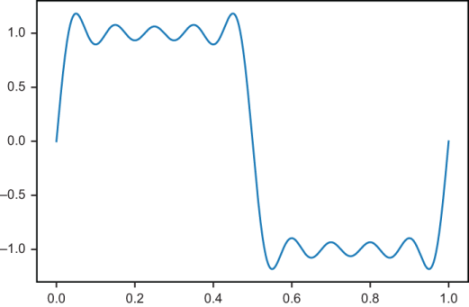
Figure 13.21 A sum of the first 5 non-zero terms of the Fourier series
This is an interesting pattern of constructive and destructive interference! Around t = 0 and t = 1, all of the sine functions are simultaneously increasing, while around t = 0.5, they are all simultaneously decreasing. This constructive interference is the dominant effect, while alternating constructive and destructive interference keeps the graph relatively flat in the other regions. With n ranging up to 19, as shown in figure 13.22, there are 10 non-zero terms and this effect is even more striking.
>>> b = [4/(n * pi) if n%2 != 0 else 0 for n in range(1,20)]
>>> f = fourier_series(0,[],b)
If we let n range all the way up to 99, we get a sum of 50 sine functions, and the function becomes nearly flat outside of a few big jumps (figure 13.23).
>>> b = [4/(n * pi) if n%2 != 0 else 0 for n in range(1,100)]
>>> f = fourier_series(0,[],b)

Figure 13.22 The first 10 non-zero terms of the Fourier series

Figure 13.23 With 99 terms, the graph of the Fourier series is nearly flat, apart from big steps at 0, 0.5, and 1.0.
If you zoom out, you can see that this Fourier series comes close to the square wave we plotted at the beginning of the chapter (figure 13.24).

Figure 13.24 The first 50 non-zero terms of the Fourier series are close to a square wave, like the first function we met in this chapter.
What we’ve done here is to build an approximation of the square wave function as a linear combination of sinusoids. It’s counterintuitive that we can do this! After all, all of the sinusoids in the Fourier series are round and smooth, and the square wave is flat and jagged. We’ll conclude this chapter by showing how to reverse engineer this approximation, starting with any periodic function and recovering the coefficients for a Fourier series that approximates it.
13.4.5 Exercises
13.5 Decomposing a sound wave into its Fourier series
Our last goal is to take an arbitrary periodic function, like the square wave, and figure out how to write it (or at least an approximation of it) as a linear combination of sinusoidal functions. This means breaking any sound wave into a combination of pure notes. As a basic example, we’ll look at a sound wave defining a chord and identify which notes make up the chord. More profoundly, we can break any sound into musical notes: a person talking, a dog barking, or a car revving its engine. Behind this result are some elegant mathematical ideas, and you now have all the background you need to understand them.
The process of breaking a function into its Fourier series is analogous to writing a vector as a linear combination of basis vectors as we did in part 1. Here’s how the analogy works. We’ll work in the vector space of functions and think of a function like the square wave, as a function of interest. Then, we’ll think of our basis as the set of functions sin(2πt), sin(4πt), sin(6πt), and so on. In section 13.3, we approximated the square wave as a linear combination beginning with
![]()
You can picture two of the basis vectors, sin(2πt) and sin(6πt), as defining two perpendicular directions in the infinite-dimensional space of functions with many other directions defined by the other basis vectors. The square wave has a component of length 4/π in the sin(2πt) direction and a component of length 4/3π in the sin(6πt) direction. These are the first two in what would be an infinite list of coordinates for the square wave in this basis (figure 13.25).

Figure 13.25 You can think of the square wave as a vector in the space of functions with a component length of 4/π in the sin(2πt) direction and component length of 4/3π in the sin(6πt) direction. The square wave has infinitely many more components beyond these two.
We can write a fourier_coefficients(f,N) function that takes a function f , which is periodic with period one, and a number N of desired coefficients. The function treats the constant function, as well as the functions cos(2nπt) and sin(2nπt) from 1 ≤ n < N, as directions in the vector space of functions and find the components of f in those directions. It returns the Fourier coefficient a0, representing the constant function, a list of Fourier coefficients a1, a2, ..., aN, and a list of Fourier coefficients b1, b2, ..., bN as a result.
13.5.1 Finding vector components with an inner product
In chapter 6, we covered how to do vector sums and scalar multiples with functions in analogy with the operations with 2D and 3D vectors. Another tool we need is an analogy for the dot product. The dot product is one example of an inner product, a way of multiplying two vectors to get a scalar that measures how aligned are the two vectors.
Let’s think back to the 3D world for a moment and show how to use the dot product to find components of a 3D vector, then we’ll do the same thing to find components of a function in the basis of sinusoidal functions. Suppose our goal is to find the components of the vector v = (3, 4, 5) in the directions of the standard basis vectors, e1 = (1, 0, 0), e2 = (0, 1, 0), and e3 = (0, 0, 1). This question is so obvious that we never put much thought into it. The components are 3, 4, and 5, respectively; that’s what the coordinates (3, 4, 5) mean!
Here, I’ll show you another way to find the components of v = (3, 4, 5) using the dot product. It’s going to be overkill because we already have the answer, but it will be useful for the case of function vectors. Notice that each of the dot products of v with a standard basis vector gives us back one of the components:
v · e1 = (3, 4, 5) · (1, 0,0) = 3 + 0 + 0 = 3
v · e2 = (3, 4, 5) · (0, 1,0) = 0 + 4 + 0 = 4
v · e3 = (3, 4, 5) · (0, 0,1) = 0 + 0 + 5 = 5
These dot products immediately tell us how to build v as a linear combination of the standard basis: v = 3e1 + 4e2 + 5e3. Be careful. This only works because the dot product agrees with our definitions of lengths and angles. Any pair of perpendicular standard basis vectors has zero dot product:
e1 · e2 = e2 · e3 = e3 · e1 = 0
And the dot products of standard basis vectors with themselves yield their (squared) lengths of one:
e1 · e1 = e2 · e2 = e3 · e3 = |e1|2 = |e2|2 = |e3|2 = 1
Another way to look at these relationships is that, according to the dot product, none of the standard basis vectors have components in the direction of the other standard basis vectors. Furthermore, each standard basis vector has component 1 in its own direction. If we want to invent an inner product to calculate components of functions, we need our basis to have the same desirable properties. In other words, we need to know that our basis functions, like sin(2πt), cos(2πt), and so on, are all perpendicular and have length 1. We’ll create an inner product for functions and test these facts.
13.5.2 Defining an inner product for periodic functions
Suppose f(t) and g(t) are two functions defined on the interval from t = 0 to t = 1, and that these repeat themselves every one unit of t. We can write the inner product of f and g as <f , g > and define it by a definite integral:

Let’s implement this in Python code, approximating the integral as a Riemann sum (as we did in chapter 8), so you can get a sense for how this inner product works like the familiar dot product. This Riemann sum defaults to 1,000 time steps as shown here:
def inner_product(f,g,N=1000):
    dt = 1/N                                    ❶
    return 2*sum([f(t)*g(t)*dt
                  for t in np.arange(0,1,dt)])  ❷
❶ The dt size defaults to 1/1000 = 0.001.
❷ For each time step, the contribution to the integral is f(t) * g(t) * dt. The integral’s result is multiplied by 2, according to the formula.
Like the dot product, this integral approximation is a sum of products of values from the input vectors. Instead of being a sum of products of coordinates, it is a sum of products of function values. You can think of a function’s values as a set of infinitely many coordinates, and this inner product as being a kind of “infinite dot product” over these coordinates.
Let’s take this inner product for a spin. For convenience, let’s define some Python functions to create the nth sine and cosine functions in our basis, and then we can test them with the inner_product function. These functions are like simplified versions of the make_sinusoid function from section 13.3.2:
def s(n):                     ❶
    def f(t):
        return sin(2*pi*n*t)
    return f

def c(n):                      ❷
    def f(t):
        return cos(2*pi*n*t)
    return f
❶ s(n) takes a whole number n and returns the function sin(2nπt).
❷ c(n) takes a whole number n and returns the function cos(2nπt).
A dot product of two 3D vectors like (1, 0, 0) and (0, 1, 0) returns zero, confirming they are perpendicular. Our inner product shows that all of our pairs’ basis functions are (approximately) perpendicular. For instance,
>>> inner_product(s(1),c(1))
4.2197487366314734e−17
>>> inner_product(s(1),s(2))
−1.4176155163484784e−18
>>> inner_product(c(3),s(10))
−1.7092447249233977e−16
These numbers are extremely close to zero, confirming that sin(2πt) and cos(2πt) are perpendicular, and sin(2πt) and sin(4πt) are perpendicular, as well as cos(6πt) and cos(20πt). Using exact integration formulas, which we won’t cover here, it’s possible to prove that for any whole numbers n and m :
〈sin(2nπt), cos(2mπt)〉 = 0
And for any pair of distinct whole numbers n and m, both
〈sin(2nπt), sin(2mπt)〉 = 0
〈cos(2nπt), cos(2mπt)〉 = 0
This is a way of saying that with respect to this inner product, all of our sinusoidal basis functions are perpendicular; none has a component in the direction of another. The other thing we need to check is that the inner product implies our basis vectors have components of 1 in their own directions. Indeed, within numerical error, this looks to be true:
>>> inner_product(s(1),s(1))
1.0000000000000002
>>> inner_product(c(1),c(1))
0.9999999999999999
>>> inner_product(c(3),c(3))
1.0
Even though we won’t go through it here, using integral formulas makes it possible to prove directly that for any whole number n
〈sin(2nπt), sin(2nπt)〉 = 1
〈cos(2nπt), cos(2nπt)〉 = 1
The last bit of tidying up we need to do is to include our constant function in this discussion. I promised before that I’d explain why we need to include a constant term in the Fourier series, and now I can give an initial explanation. The constant function is required to build a complete basis of functions; not including this would be like omitting e2 from the basis for 3D space and going forward with e1 and e3. If you did that, there’d be functions you simply couldn’t build out of basis vectors.
Any constant function is perpendicular to every sine and cosine function in our basis, but we need to pick the value of the constant function so that it has component 1 in its own direction. That is, if we implement a Python function const(t), we should find that inner_product(const,const) returns 1. The right constant value for const to return turns out to be 1/√2 (and you can check in the following exercise that this value makes sense!):
from math import sqrt

def const(n):
    return 1 /sqrt(2)
With this defined, we can confirm the constant function has the right properties:
>>> inner_product(const,s(1))
−2.2580204307905138e−17
>>> inner_product(const,c(1))
−3.404394821604484e−17
>>> inner_product(const,const)
1.0000000000000007
We now have the tools we need to find the Fourier coefficients of a periodic function. These coefficients are nothing more than components of the function in the basis we’ve defined.
13.5.3 Writing a function to find Fourier coefficients
In the 3D example, we saw that the dot product of a vector v with a basis vector e i gave us the component of v in the direction of e i. We’ll use the same process for a periodic function f .
The coefficients an for n ≥ 1 tell us the components of f in the direction of the basis function cos(2nπt). They are computed as the inner products of f with these basis functions:
an = 〈f, cos(2nπt)〉 , n ≥ 1
Likewise, every Fourier coefficient bn tells us the component of f in the direction of a basis function sin(2nπt) and can also be computed with an inner product:
bn = 〈f, sin(2nπt)〉
Finally, the number a 0 is the inner product of f with the constant function, whose value is 1/√2. All of these Fourier coefficients can be computed with Python functions we’ve already written, so we’re ready to assemble the fourier_coefficients function we set out to write. Remember, the first argument to the function is the function we want to analyze, and the second argument is the maximum number of sine and cosine terms we want:
def fourier_coefficients(f,N):
    a0 = inner_product(f,const)     ❶
    an = [inner_product(f,c(n))
          for n in range(1,N+1)]    ❷
    bn = [inner_product(f,s(n))
          for n in range(1,N+1)]    ❸
    return a0, an, bn
❶ The constant term a0 is the inner product of f with the constant basis function.
❷ The coefficients an are given by inner products of f with cos(2nπt) for 1 < n < N + 1.
❸ The coefficients bn are given by inner products of f with sin(2nπt) for 1 ≤ n < N + 1.
As a sanity check, a Fourier series should give back its own coefficients. For instance
>>> f = fourier_series(0,[2,3,4],[5,6,7])
>>> fourier_coefficients(f,3)
(−3.812922200197022e−15,
 [1.9999999999999887, 2.999999999999999, 4.0],
 [5.000000000000002, 6.000000000000001, 7.0000000000000036])
Note If you want the inputs and outputs to match non-zero constant terms, you need to revise the const function to be f(t) = 1/√2 instead of f(t) = 1. See exercise 13.8.
Now that we can automatically compute Fourier coefficients, we can conclude our exploration by building some Fourier approximations of interestingly shaped periodic functions.
13.5.4 Finding the Fourier coefficients for the square wave
We saw in the last section that the Fourier coefficients for the square wave were all zero except for the bn coefficients for odd n values. That is, the Fourier series is built as a linear combination of the function sin(2nπt) for odd values of n. For odd n, the coefficient was bn = 4/nπ. I didn’t explain why those were the coefficients, but now we can check our work.
To make a square wave that repeats itself every unit of t, we can use the value t%1 in Python, which computes the fractional part of t. Because, for example, 2.3 % 1 is 0.3 and 0.3 % 1 is 0.3, a function written in terms of t % 1 is automatically periodic with the period 1. The square wave has a value of +1 when t % 1 < 0.5 and −1 otherwise
def square(t):
    return 1 if (t%1) < 0.5 else −1
Let’s look at the first 10 Fourier coefficients for this square wave. Run
a0, a, b = fourier_coefficients(square,10)
and you’ll see that a0 and the entries of a are all small, as with every other entry of b. The values of b1, b3, b5, and so on are represented by b[0], b[2], b[4], ..., because Python arrays are zero-indexed. These are all close to the expected values:
>>> b[0], 4/pi
(1.273235355942202, 1.2732395447351628)
>>> b[2], 4/(3*pi)
(0.4244006151333577, 0.4244131815783876)
>>> b[4], 4/(5*pi)
(0.2546269646514865, 0.25464790894703254)
We already saw that a Fourier series with these coefficients is a solid approximation of the square wave graph. Let’s conclude this section by looking at two example functions we haven’t seen before and plotting the Fourier series alongside the original functions to show that the approximation works.
13.5.5 Fourier coefficients for other waveforms
Next, we consider more functions beyond the square wave graph that can be modeled using a Fourier transform. Figure 13.26 shows a new, interestingly shaped waveform called a sawtooth wave.

Figure 13.26 A sawtooth wave plotted over five periods
On the intervals from t = 0 to t = 1, the sawtooth wave is identical to the function f(t) = t and then it repeats itself every one unit. To define the sawtooth wave as a Python function, we can simply write
def sawtooth(t):
    return t%1
To see its Fourier series approximation with up to 10 sine and cosine terms, we can plug the Fourier coefficients directly into our Fourier series function. Plotting it alongside the sawtooth, as shown in figure 13.27, we can see it has a good fit.
>>> approx = fourier_series(*fourier_coefficients(sawtooth,10))
>>> plot_function(sawtooth,0,5)
>>> plot_function(approx,0,5)

Figure 13.27 The original sawtooth wave from figure 13.26 with its Fourier series approximation
Once again, it’s striking how close we can come to a function with sharp corners using only a linear combination of smooth sine and cosine waves. This function happens to have a non-zero constant coefficient a0. That’s required because this function only has values above zero, while sine and cosine functions contribute negative values.
As a final example, take a look at the following function defined as speedbumps(t) in the source code for this book. Figure 13.28 shows the graph.

Figure 13.28 The speedbumps(t) function that alternates between flat stretches and round bumps
The implementation of this function isn’t important, but this one is an interesting example because it has non-zero coefficients for the cosine functions and all zeros for the sines. Even with 10 terms, we get a good approximation. Figure 13.29 shows the graph of the Fourier series with a0 and ten cosine terms (the coefficients bn are all zero).
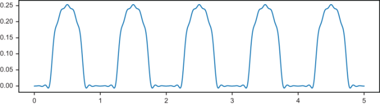
Figure 13.29 The constant term and first 10 cosine terms for the Fourier series of the speedbumps(t) function
You can see some wobbles when we graph these approximations, but when these waveforms are translated to sound, the Fourier series can be good enough. Because we are able to transform waveforms of all shapes to lists of their Fourier coefficients, we can store and transmit audio files efficiently.
13.5.6 Exercises
|
a1 = v · u1 = (3, 4, 5) · (2, 0, 0) = 6 a2 = v · u2 = (3, 4, 5) · (0, 1, 1) = 9 a3 = v · u3 = (3, 4, 5) · (1, 0,−1) = −2 |
|
|

def modified_sawtooth(t):
    return 8000 * sawtooth(441*t)
arr = sample(modified_sawtooth,0,1,44100)
sound = pygame.sndarray.make_sound(arr)
sound.play()
|
Summary
-
Sound waves are pressure changes over time that propagate through the air to our ears where we perceive these as sounds. We can represent a sound wave as a function that loosely represents the change in air pressure over time.
-
PyGame and most other digital audio systems used sampled audio. Rather than a function defining a sound wave, these systems use arrays of values of the function taken at uniform intervals. For instance, CD audio commonly uses 44,100 values for each second of audio.
-
Sound waves with random shapes sound like noise, while waves with shapes that repeat on fixed intervals produce well-defined musical notes. A function that repeats its values on a certain interval is called a periodic function.
-
The sine and cosine functions are periodic functions, and their graphs repeat curved shapes called sinusoids.
-
Sine and cosine repeat their values every 2π units. That value is called their period. The frequency of a periodic function is the reciprocal of the period, which is 1/(2π) for sine and cosine.
-
A function of the form sin(2nπt) or cos(2nπt) has frequency n. High frequency sound wave functions produce high-pitched musical notes.
-
The maximum height of a periodic function is called its amplitude. Multiplying a sine or cosine function by a number increases the amplitude of the function and the volume of the corresponding sound wave.
-
To create the effect of two sounds playing at once, you can add the functions that define their corresponding sound waves to create a new function and a new sound wave. Generally, you can take any linear combination of existing sound waves to create a new sound wave.
-
A linear combination of a constant function along with functions of the form sin(2nπt) and cos(2nπt) for various values of n is called a Fourier series. Despite being built out of smooth sine and cosine functions, Fourier series can be good approximations for any periodic functions, even those with sharp corners like square waves.
-
You can think of the constant function along with the sines and cosines at different frequencies as a basis for the vector space of periodic functions. The linear combination of these basis vectors that best approximate a given function are called Fourier coefficients.
-
We can use the dot product of a 2D or 3D vector with a standard basis vector to find its component in the direction of that basis vector.
-
Analogously, we can take a special inner product of a periodic function with a sine or cosine function to find a component associated with that function. The inner product for periodic functions is a definite integral taken over a specified range, in our case, from zero to one.