
Noise Factors Overview
Noise factors (robust process engineering) enables you to produce acceptable products reliably, despite variation in the process variables. Even when your experiment has controllable factors, there is a certain amount of uncontrollable variation in the factors that affects the response. This is called transmitted variation. Factors with this variation are called noise factors. You cannot control some factors, like environmental noise factors. The mean for some factors can be controlled, but their standard deviation is uncontrollable. This is often the case for intermediate factors that are output from a different process or manufacturing step.
A good approach to making the process robust is to match the target at the flattest place of the noise response surface. Then, the noise has little influence on the process. Mathematically, this is the value where the first derivatives of each response with respect to each noise factor are zero. JMP computes the derivatives for you.
To analyze a model with noise factors:
1. Fit the appropriate model (for example, using the Fit Model platform).
2. Save the model to the data table with the Save > Prediction Formula command.
3. Launch the Profiler (from the Graph menu).
4. Assign the prediction formula to the Y, Prediction Formula role and the noise factors to the Noise Factor role.
5. Click OK.
The resulting profiler shows response functions and their appropriate derivatives with respect to the noise factors, with the derivatives set to have maximum desirability at zero.
6. Select Maximize Desirability from the Profiler menu.
This finds the best settings of the factors, balanced with respect to minimizing transmitted variation from the noise factors.
Example
As an example, use the Tiretread.jmp sample data set. This data set shows the results of a tire manufacturer’s experiment whose objective is to match a target value of HARDNESS= 70 based on three factors: SILICA, SILANE, and SULFUR content. Suppose the SILANE and SULFUR content are easily (and precisely) controllable, but SILICA expresses variability that is worth considering.
For comparison, first optimize the factors for hardness without considering variation from the noise factor.
1. Select Graph > Profiler to launch the Profiler.
2. Assign Pred Formula HARDNESS to the Y, Prediction Formula role.
3. Click OK.
4. Select Desirability Functions in the Prediction Profiler menu.
5. Double-click in the Desirability plot to open the Response Goal window. Select Match Target from the list.
6. Select Maximize Desirability to find the optimum factor settings for our target value of HARDNESS.
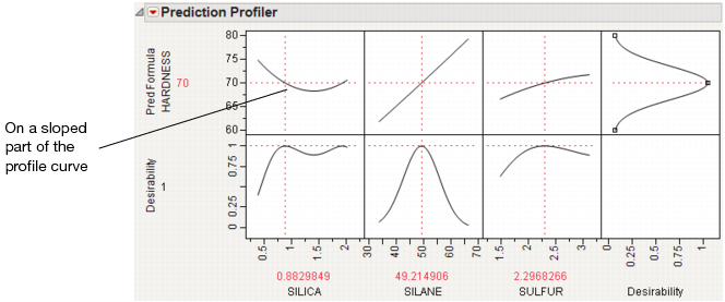
We get the following Profiler display. Notice that the SILICA factor’s optimum value is on a sloped part of a profile curve. This means that variations in SILICA are transmitted to become variations in the response, HARDNESS.
Note: You might get different results from these because different combinations of factor values can all hit the target.
Figure 9.2 Maximizing Desirability for HARDNESS
Now, we would like to not just optimize for a specific target value of HARDNESS, but also be on a flat part of the curve with respect to Silica. So, repeat the process and add SILICA as a noise factor.
1. Select Graph > Profiler.
2. Select Pred Formula HARDNESS and click Y, Prediction Formula.
3. Select SILICA and click Noise Factors.
4. Click OK.
5. Change the Pred Formula Hardness desirability function as before.
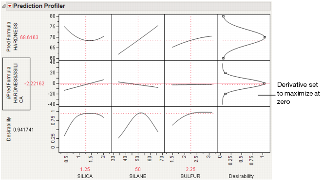
The resulting profiler has the appropriate derivative of the fitted model with respect to the noise factor, set to be maximized at zero, its flattest point.
Figure 9.3 Derivative of the Prediction Formula with Respect to Silica
6. Select Maximize Desirability to find the optimum values for the process factor, balancing for the noise factor.
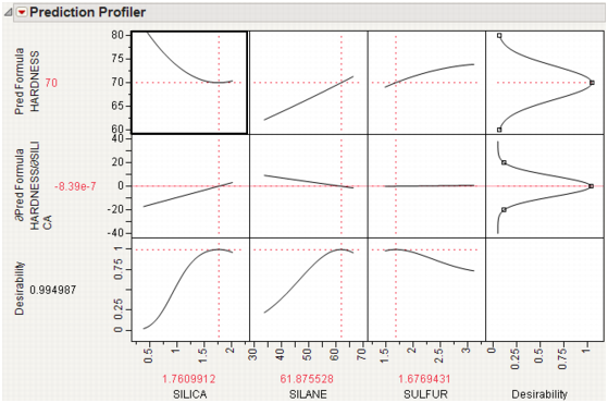
This time, we have also hit the targeted value of HARDNESS, but our value of SILICA is on its flatter region. This means variation in SILICA does not transmit as much variation to HARDNESS.
Figure 9.4 Maximize Desirability
You can see the effect this has on the variance of the predictions by following these steps for each profiler (one without the noise factor, and one with the noise factor):
1. Select Simulator from the platform menu.
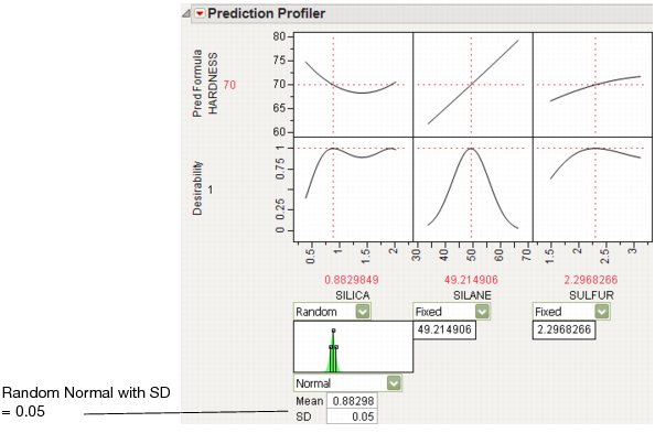
2. Assign SILICA to have a random Normal distribution with a standard deviation of 0.05.
Figure 9.5 Setting a Random Normal Distribution
3. Click Simulate.
4. Click the Make Table button under the Simulate to Table node.
Doing these steps for both the original and noise-factor-optimal simulations results in two similar data tables, each holding a simulation. In order to make two comparable histograms of the predictions, we need the two prediction columns in a single data table.
5. Copy the Pred Formula HARDNESS column from one of the simulation tables into the other table. They must have different names, like Without Noise Factor and With Noise Factor.
6. Select Analyze > Distribution and assign both prediction columns as Y.
7. When the histograms appear, select Uniform Scaling from the Distribution main title bar.
Figure 9.6 Comparison of Distributions with and without Noise Factors
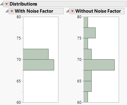
The histograms show that there is much more variation in Hardness when the noise factor was not included in the analysis.
It is also interesting to note the shape of the histogram when the noise factor was included. In the comparison histograms above, note that the With Noise Factor distribution has data trailing off in only one direction. The predictions are skewed because Hardness is at a minimum with respect to SILICA, as shown in Figure 9.7. Therefore, variation in SILICA can make only HARDNESS increase. When the non-robust solution is used, the variation could be transmitted either way.
Figure 9.7 Profiler Showing the Minima of HARDNESS by SILICA
Noise Factors in Other Platforms
Noise factor optimization is also available in the Contour Profiler, Custom Profiler, and Mixture Profiler. See the “Contour Profiler” chapter, the “Custom Profiler” chapter, and the “Mixture Profiler” chapter.
..................Content has been hidden....................
You can't read the all page of ebook, please click here login for view all page.