
3
Experimental Designs for Formulations
“Experiment... day and night. Experiment and it will lead you to the light.”
Cole Porter
Overview
We have seen how the experimental regions and models for experiments with formulations differ from traditional approaches involving unconstrained variables. In this chapter we review basic experimental designs that are most frequently used in practice, such as those based on the simplex. In the next chapter, we review basic models used to analyze data from these types of experiments. In subsequent chapters, we will present designs and models for more complex situations, such as with constrained components, or experiments with both formulation and process variables.
CHAPTER CONTENTS
3.1 Geometry of the Experimental Region
3.5 Summary and Looking Forward
3.1 Geometry of the Experimental Region
As discussed in Chapter 1, experiments with formulations have some important differences from experiments involving variables that can be changed independently of each other. There are two basic reasons for these differences. First, formulation experiments have constraints in that the proportion of each component must be bounded by 0 and 1.0--i.e., 0 ≤ xi ≤ 1.0. Second, the components collectively must sum to 1.0--i.e., ∑nixi=1.0. We saw in Figure 1.1 that the summation constraint has the effect of modifying the geometry of the experimental region and reducing the dimensionality. Recall that for two independent variables (non-formulations), the typical factorial designs are based on a two-dimensional square. With formulations, however, the second component must be one minus the first component. Hence, the available design space becomes a line instead of a square. Therefore, there is only one true dimension in the formulation design space, or one fewer than the dimensionality of the factorial space.
When one is experimenting with three independent (non-formulation) variables, the typical factorial designs are based on a three-dimensional cube. However, since three formulation components must sum to 1.0, once the proportions of the first two components have been determined, the third must be 1.0 minus these. Therefore, the available design space becomes a two-dimensional triangle, or simplex. Rather than graph this simplex in three-dimensional space, experimenters typically graph it in two-dimensional space, as if one were looking down on the simplex plane from a position perpendicular to it.
Figure 3.1 shows a three-dimensional simplex, or tetrahedron, composed of four components. Again, the axis for x1 runs from the center of the base of the simplex to the top vertex, and the axes for x2, x3, and x4 run similarly, from the center of each base of the tetrahedron to the opposite vertex. Mathematically, such geometric shapes can be defined in any dimensionality. Hence, experimental designs based on simplexes can be used in higher dimensions. Of course, they are not easy to graph.
Figure 3.1 – Simplex with Four Components

3.2 Basic Simplex Designs
As discussed in Chapter 2, a key principle of experimental design is that designs and statistical models go hand in hand. That is, experimenters generally design experiments to enable estimation of models of potential interest. Once the design has been executed, the options for modeling the data produced from this particular design will be limited. We discuss basic simplex designs in this chapter, and then discuss the typical models fit to the resulting data in Chapter 4. However, keep in mind that in practice selection of design and selection of model need to be considered concurrently rather than consecutively. As noted in Chapter 2, a sequential strategy for design and model building facilitates such an approach.
The most basic simplex designs allow the experimenter to cover the entire available design space--that is, to vary each component from 0 to 1.0. In subsequent chapters we discuss situations where the entire design space is not of interest and how to address them. For example, few people would be interested in a salad dressing made of 100% vinegar. Figure 3.2 shows the points in what is called a simplex-centroid design with three components. While not the only or necessarily the best option, this is a common design used with formulations. Note that it has points run at each of the vertices (pure blends), midpoints on each side of the simplex (50-50 blends), and a point at the centroid, or middle of the simplex. This requires only seven formulations to be run, and therefore allows up to seven parameters to be estimated in the subsequent model. Such a model allows for inclusion of terms to account for curvature, or non-linear blending, to which we return in Chapter 4.
Figure 3.2 – Simplex-Centroid with Three Components

In general, a full simplex-centroid design involving q components will have q pure blends, (q2) 50-50 blends involving two components, (q3) 1/3-1/3-1/3 blends involving three components, (q4) .25-.25-.25-.25 blends involving four components, and so on, up to (qq)--i.e., one, 1/q-1/q-...1/q centroid. Note that (qi) means the number of combinations, or distinct ways of choosing i components from q. Mathematically, (qi)=q!i!(q−i)!′ where n! = n*(n-1)*(n-2)*(n-3)*...*1. A full simplex-centroid design has 2q - 1 runs total (Cornell 2011). Therefore, this design can require an impractical number for points for larger formulations. For example, if we have seven components, a full simplex centroid design would require 27 – 1 = 127 runs. In practice, therefore, experimenters often run a reduced simplex-centroid design, including only the q pure blends, (q2) 50-50 blends, and one centroid. Figure 3.3 shows a reduced simplex-centroid design with four components.
Figure 3.3– Reduced Simplex-Centroid Design for Four Components

The design sizes, in terms of number of points in the experiment (n), for different numbers of components (q) from three to ten, both for the full and reduced simplex-centroid (SC), are shown in Table 3.1, assuming no replication. It is clear that if we experiment with more than four components, the reduced simplex-centroid designs are considerably more economical. Going forward, we focus on the reduced simplex-centroid design. Hence, we will simply use the term simplex-centroid to refer to this reduced design.
Table 3.1 – Simplex-Centroid Design Sizes
| Components (q) | Points - Full SC (n) | Points - Reduced SC (n) |
| 3 | 7 | 7 |
| 4 | 15 | 11 |
| 5 | 31 | 16 |
| 6 | 63 | 22 |
| 7 | 127 | 29 |
| 8 | 255 | 37 |
| 9 | 511 | 46 |
| 10 | 1023 | 56 |
Note that the additional number of points required as components are added increases with q. That is, for the full simplex-centroid the design size doubles, plus one, with each new component added. Conversely, the reduced simplex-centroid design size increases by one more each time. That is, the difference between three and four component designs is four points, between four and five component designs it is five points, and so on.
As noted in Chapter 2, replication is very useful in experimental design, both to reduce overall uncertainty, as well as to obtain a better estimate of experimental error. Of course, replicating the entire experiment doubles the design size. Therefore, experimenters often run two to three points at the centroid of the design, in order to provide more accurate prediction in the center of the design, or perhaps at pure blends, to enable better estimation of model coefficients. Such replication increases the overall size of the design, but not nearly as much as full replication. See Cornell (2002, 2011) for a more detailed discussion of replication strategies.
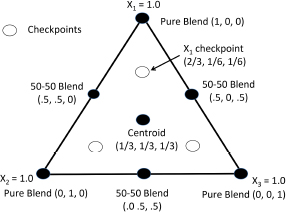
Note that both types of simplex-centroid designs put all experimental points except the centroid on the exterior of the design space--i.e., with at least one component at zero. Therefore, besides running replicates at the centroid or pure blends, another option for using additional experimental runs is to include points halfway between the centroid and the pure blends. Such points are often referred to as checkpoints because they enable experimenters to check the fit of the model in the interior of the design space--for example with a model based solely on the n points in the simplex-centroid design.
For example, with three components these checkpoints would be at (2/3, 1/6, 1/6), (1/6, 2/3, 1/6), and (1/6, 1/6, 2/3). This simplex-centroid design with checkpoints is shown in Figure 3.4. Note that 2/3 is halfway between 1/3, the level of each component at the centroid, and 1.0, the level of the pure blend in that component. This was the design used in both the vegetable oil and placebo tablet experiments presented in Chapter 1. Obviously, the inclusion of checkpoints adds q points to the design sizes shown in Table 3.1. The additional points enable estimation of more terms in the subsequent model (for example, if severe curvature is present, more polynomial terms might be required to adequately fit the data). Models that are appropriate for each design that is discussed in this chapter will be presented in Chapter 4.
Figure 3.4 – Simplex-Centroid Design with Checkpoints: Three Components
3.3 Screening Designs
As noted in Chapter 2, experimental design and analysis are best done in a sequential fashion, in which each round of design and analysis answers some questions, but perhaps raises new ones as well. Some aspects of the existing subject matter theory may be validated, but surprises that challenge our current theories may also be observed. The scientific method integrates data with subject matter knowledge in a continual cycle of validating or challenging theories with data. Creative thought leads to new or modified theories, which explain the observed data, and understanding of the phenomenon of interest thereby advances.
Subsequent experimental designs can take advantage of what has been learned previously and focus on the remaining unanswered questions. In this way, experimenters can use hindsight to their advantage--i.e., to use what has been learned through previous experiments to guide the next round of experimentation. The cycle of the scientific method continues. This sequential approach to the scientific method is critical in selecting experimental designs, since the most appropriate design depends on the current phase in which experimenters find themselves--i.e., the specific phase in the overall roadmap for experimentation discussed in Chapter 2.
If the experimenter is in the screening phase, with a large number of potential components, a simplex-centroid design with or without checkpoints may not be practical. For example, if there were ten potential components of interest, a simplex-centroid design would require 56 points (see Table 3.1), and adding checkpoints would bring the design up to 66 points. Running an experiment with 66 points is usually challenging from a practical point of view. In such situations, running a smaller screening experiment first, to simply identify the most important components, may be a more effective strategy.
In this case, the experimenter could run a 25-point screening design (Snee and Marquardt 1976) to identify the most critical components. Hypothetically, this could point to identification of four components that were most critical. Then, the other six components could be held constant or combined in future experimentation. A simplex-centroid design in four components would require only 11 points, or 15 with checkpoints. Therefore, two full experiments could be run with a total of 36 points (40 with checkpoints), while a simplex-centroid design in ten components would require 56 points (66 with checkpoints).
In addition to reducing the total experimental effort by over a third, the sequential approach would enable the second design to take advantage of all insight gained from the first design, such as the most promising levels of the variables of interest.
Of course, there is no guarantee that the screening experiment will produce exactly four critical components; the scientific method and statistical strategies based on it are difficult to precisely forecast. However, experience in a wide variety of application areas, including those involving formulations, has shown that most processes have a relatively small number of critical factors. In other words, the sequential strategy discussed in Chapter 2 has been proven effective by a large number of researchers over several decades. Such a strategy does not guarantee success, but puts the odds in the experimenter’s favor.
A typical screening design uses multiple points in a line from 0 to 1.0 for each component, to enable evaluation of the overall impact of that component on the response of interest, while holding the other variables in constant proportion to one another. Table 3.2 shows the simplex-screening designs suggested by Snee and Marquardt (1976) requiring 2q + 1 points.
Table 3.2 – Simplex-Screening Designs (2q + 1)
| Type of Point | Level of xi | Level of Other x’s | Number of Such Points |
| Vertices | 1.0 | 0 | q |
| Interior | (q+1)/2q | 1/2q | q |
| Centroid | 1/q | 1/q | 1 |
For q=3, this screening design consists of the seven points shown in Figure 3.5. Note that this is a simplex-centroid design with checkpoints, but without the 50-50 blends. Note also that there are three points along each axis, for x1, x2, and x3. As x1 increases from 1/3 to 2/3 to 1.0, x2 and x3 remain in equal proportion. That is, for each of these points on the x1 axis, x2 = x3. The same principle is true along the x2 and x3 axes. Therefore, if we measure changes in the response y as we move along these axes, this change can be attributed to the impact of increasing this particular variable--x1 in this case. Of course, in formulation systems, increasing one component by definition means decreasing others. When moving along the component axes, however, the proportions of the other components are held constant relative to each other, simplifying interpretation. We discuss interpretation of screening designs more fully in Chapter 5.
Figure 3.5 – 2q + 1 Simplex-Screening Design for Three Components

Snee and Marquardt (1976) also noted that when experimenters suspect that blending behavior will change dramatically if an ingredient is totally absent from the formulation, that q additional “End Effect” points could be included--that is, with this xi = 0, and all other components set to 1/(q-1). Such a point would be included for all q components, bringing the total design size up to 3q + 1. In the case of q = 3, these points would in fact be the 50-50 blends from the simplex-centroid design. Note that while a 3q + 1 simplex-screening design is equivalent to a simplex-centroid design with checkpoints in the case of q = 3, this is not the case in general. As q increases, the differences between the simplex-centroid designs from Table 3.1 and the 2q + 1 and 3q + 1 simplex-screening designs become more dramatic, as illustrated in Table 3.3.
Table 3.3 – Sizes of Simplex-Centroid (SC) and Simplex-Screening (SS) Designs
| q | SC (No Checkpoints) |
SC (Checkpoints) |
SS (2q + 1) |
SS (3q + 1) |
(SC No C) – (2q + 1) |
| 3 | 7 | 10 | 7 | 10 | 0 |
| 4 | 11 | 15 | 9 | 13 | 2 |
| 5 | 16 | 21 | 11 | 16 | 5 |
| 6 | 22 | 28 | 13 | 19 | 9 |
| 7 | 29 | 36 | 15 | 22 | 14 |
| 8 | 37 | 45 | 17 | 25 | 20 |
| 9 | 46 | 55 | 19 | 28 | 27 |
| 10 | 56 | 66 | 21 | 31 | 35 |
Note that the last column in Table 3.3 shows the difference in the number of points required by a simplex-centroid design with no checkpoints versus a 2q + 1 simplex-screening design (or between a simplex-centroid with checkpoints versus a 3q + 1 simplex-screening design). As we have seen, there is no difference with three components, but with four or more components there is a difference. When one is experimenting with eight or more components, the difference is clearly of significant practical importance. Initial use of screening designs when considering large numbers of components can therefore prove to be an effective strategy.
3.4 Response Surface Designs
As noted in Chapter 2, experimenters often begin investigations with screening designs to identify the most critical components. Those that do not appear to be critical may be held constant in subsequent experiments, or perhaps combined with other components that have roughly equivalent effects. A second round of experimentation and modeling may then focus on the critical components identified, perhaps using a simplex-centroid design with or without checkpoints. Once the key components have been identified, and the most promising regions of the design have been identified, an additional round of experimentation and modeling may be used. This round could be used in developing an adequate model to optimize the response or responses. Such a model would, of course, require accounting for all non-linear blending--i.e., curvature--present.
In such circumstances, experimenters may use designs specifically structured to estimate non-linear blending. These designs are typically larger than simplex-centroid and simplex-screening designs, and they are often referred to as response surface designs because they are used to develop good estimation of the overall response surface, or functional form of the response. A class of designs referred to as simplex-lattice designs are a common choice for estimating such response surfaces. The term lattice refers to a uniformly spaced distribution of points on the simplex. Cornell (2011) used the notation (q,m) simplex-lattice to refer to a lattice design in q components to enable estimation of a polynomial of degree m. For example, each component xi might take on m + 1 distinct values, at the levels: 0, 1/m, 2/m, .....1. The (q,m) simplex-lattice design would then consist of all possible combinations (formulations) where these proportions are used. More recently, computer-aided designs--discussed further in Part 3--have been used for response surface designs.
Figure 3.6 shows both (3,3) and (4,3) simplex-lattice designs. Because it is difficult to visualize the (4,3) design, we list this design in Table 3.4. The (3,3) design has three components and enables estimation of a third-order polynomial--that is, one including terms such as x1x2x3. The (4,3) design is also intended to enable estimation of cubic terms, but in this case with four components in the mixture. Both designs have m + 1 = 4 distinct levels of each component, which are 0, 1/3, 2/3, and 1.0. First order polynomials would include only linear terms, and they would not account for any curvature. Second order polynomials incorporate some ability to account for curvature in general. Third order polynomials are more flexible relative to curvature, and they suffice for most practical problems. Of course, there are unique problems with more complex non-linear blending requiring more advanced approaches.
Figure 3.6 – (3,3) and (4,3) Simplex-Lattice Response Surface Designs

Table 3.4 – The (4,3) Simplex-Lattice Design
| Component Levels | Components Levels | ||||||||
| Point | X1 | X2 | X3 | X4 | Point | X1 | X2 | X3 | X4 |
| 1 | 1.0 | 0.0 | 0.0 | 0.0 | 11 | 1/3 | 0.0 | 0.0 | 2/3 |
| 2 | 0.0 | 1.0 | 0.0 | 0.0 | 12 | 2/3 | 1/3 | 0.0 | 0.0 |
| 3 | 0.0 | 0.0 | 1.0 | 0.0 | 13 | 2/3 | 0.0 | 1/3 | 0.0 |
| 4 | 0.0 | 0.0 | 0.0 | 1.0 | 14 | 2/3 | 0.0 | 0.0 | 1/3 |
| 5 | 0.0 | 1/3 | 1/3 | 1/3 | 15 | 0.0 | 1/3 | 2/3 | 0.0 |
| 6 | 1/3 | 0.0 | 1/3 | 1/3 | 16 | 0.0 | 1/3 | 0.0 | 2/3 |
| 7 | 1/3 | 1/3 | 0.0 | 1/3 | 17 | 0.0 | 0.0 | 1/3 | 2/3 |
| 8 | 1/3 | 1/3 | 1/3 | 0.0 | 18 | 0.0 | 2/3 | 1/3 | 0.0 |
| 9 | 1/3 | 2/3 | 0.0 | 0.0 | 19 | 0.0 | 2/3 | 0.0 | 1/3 |
| 10 | 1/3 | 0.0 | 2/3 | 0.0 | 20 | 0.0 | 0.0 | 2/3 | 1/3 |
The number of points in a (q,m) simplex-lattice design is (q+m−1 m), which is equal to (q+m-1)!/m!(q-1)! Note that m! means m factorial and is mathematically defined as m(m-1)(m-2)....1. For example, the number of points in a (4,3) simplex is (63) = 6!/3!3! = 6*5*4/3*2*1 = 120/6 = 20. Table 3.5 shows the number of points in common (q,m) simplex-lattice designs.
Table 3.5 – Number of Points in (q,m) Simplex-Lattice Designs
| Components (q) | |||||
| Degree (m) | 3 | 4 | 5 | 6 | 7 |
| 1 | 3 | 4 | 5 | 6 | 7 |
| 2 | 6 | 10 | 15 | 21 | 28 |
| 3 | 10 | 20 | 35 | 56 | 84 |
| 4 | 15 | 35 | 70 | 126 | 210 |
Note that the (q,1) simplex-lattice design incorporates only two levels for each component, 0 and 1. Therefore, it includes only the pure blends, with one component at 1 and all others at 0. Hence, it has only q points. This is not a design used commonly in practice, as it neither provides information about the interior of the design nor enables understanding of how the components blend. It is listed here primarily for completeness.
Simplex-lattice designs can either be constructed using statistical software applications such as JMP, or with spreadsheets such as Excel, or by hand. To construct them by hand, experimenters would consider all possible combinations of the levels of the xi, such as 0, 1/m, 2/m, and so on, but of course include only those points for which the components sum to 1.0. Consider the case of q = 3 and m = 3, which is the three-component design depicted in Figure 3.6. Each component takes on the four levels: 0, 1/3, 2/3, and 1.0. However, among all possible combinations of these four levels using the three components, only those shown on the left side of Figure 3.6 sum to 1.0. Hence, these comprise the (3,3) simplex-lattice design. Potential combinations of these levels such as (2/3, 2/3, 1/3) do not sum to 1.0, and therefore they are not included in the design.
3.5 Summary and Looking Forward
In this chapter we have covered basic formulation designs for evaluation of complete formulation design spaces--that is, spaces in which each component can be varied over its full range from 0 to 1.0. We noted that, with formulations, the constraints on the individual components and their sum produce a design space that is very different from the typical cuboidal spaces used with independent (non-formulation) variables. The design space with components that can be varied from 0 to 1.0 is a tetrahedron, or simplex, and relies on triangular coordinates. Therefore, a different approach to design is required versus the more common factorial designs.
The most basic designs cover the vertices, or pure blends, typically with 50-50 edge-points and a center point, or centroid, as well. Such designs are referred to as simplex-centroid designs. We also considered screening designs that are useful in identifying the most critical components from among a large candidate list. Such designs are much smaller than the full simplex-centroid designs, and therefore they fit into the sequential experimentation strategy discussed in Chapter 2. Once the critical components have been identified and the most promising levels of the components, response surface designs that enable estimation of polynomial models are often used. Such designs are useful in optimizing one or more responses using empirical models. Of course, these are not the only possible designs that can be used with formulations.
In Part 3 of this book--that is, Chapters 6 through 8--we discuss the common situation where there are limitations on the levels of the components, resulting in the feasible design space being smaller than the entire simplex. In particular, we consider cases where the geometric shape of the design space is irregular, and difficult to visualize. Computer-aided approaches that first quantify the feasible design space and then develop appropriate designs to model the responses within this space are typically required. We now discuss in further detail the models most often used with formulation data. As with design, there are important differences in formulation models relative to models involving only independent variables. In Chapter 9, we discuss experimental strategies including both formulation and process (non-formulation) variables.
3.6 References
Cornell, J.A. (2002) Experiments with Mixtures: Designs, Models, and the Analysis of Mixture Data, 3rd Edition, John Wiley & Sons, New York, NY.
Cornell, J.A. (2011) A Primer on Experiments with Mixtures, John Wiley & Sons, Hoboken, NJ.
Snee, R.D., and Marquardt, D.W. (1976) “Screening Concepts and Designs for Experiments with Mixtures.” Technometrics, 18 (1), 19-29.