6
Experiments with Single and Multiple Component Constraints

";When life gives you lemons, make lemonade.";

Elbert Hubbard (1915)

Overview

Part 2 of this text covered basic design and analysis of experiments with formulations. Components could vary from 0 to 100% of the blend. In Part 3, which begins with this chapter, we discuss how to address the common situation where there are constraints on the levels of the components. At first one might be concerned about the added complexity created by the constraints, but component constraints are a reality. As the opening quotation suggests, we must find a way to deal with the constraints, and we do that in the chapter. We will discuss how upper and lower bounds on the components affect the region of experimentation and how to construct formulation experiments in this situation. We also address the situation where, in addition to upper and lower bounds on the components, there may also be multiple component constraints that have to be considered. Our discussion includes how to develop models for the data and how to interpret response surface contour plots of the predicted responses to select useful formulations.  We focus on three and four component systems to help understand the issues involved, as these are easier to graph. In Chapter 8 we will discuss response surface experiments involving more components.

CHAPTER CONTENTS

Overview

6.1 Component Constraints

6.2 Components with Lower Bounds

6.3 Three-Component Example

6.4 Computation of the Extreme Vertices

6.5 Midpoints of Long Edges

6.6 Sustained Release Tablet Development - Three Components

6.7 Four-Component Flare Experiment

Computation of the Vertices

Number of Blends Required

Addition of the Constraint Plane Centroids

Regions with Long Edges

Evaluation of the Results

6.8 Graphical Display of a Four-Component Formulation Space

6.9 Identification of Clusters of Vertices

6.10 Construction of Extreme Vertices Designs for Quadratic Formulation Models

Replication and Assessing Model Lack of Fit

6.11 Designs for Formulation Systems with Multicomponent Constraints

6.12 Sustained Release Tablet Formulation Study

6.13 Summary and Looking Forward

6.14 References

6.1 Component Constraints

In many formulation experiments it is not possible to explore the total theoretical range (0 to 100%) of all the components. For example, in the rocket propellant example seen earlier, it is not possible to make a propellant without fuel. Another example of a formulation with constraints comes from the development of an aerosol propellant. In this project the team, which included Ron Snee, found that one of the components had upper and lower bounds because of pressure restrictions. Another component had upper restrictions because of a flammability constraint; if the amount of the component got above 30%, the aerosol would be flammable. Solubility constraints were also encountered in developing the formulation.

In these situations, the region available for experimentation consists only of a subset of the total simplex space. In some situations, physical and economic considerations result in lower (a_i) and/or upper (b_i) constraints on one or more of the q components in the formulation. For example, the feasible level of component x_i may be constrained to the following:

0 < a_i < x_i < b_i < 1

Constructing effective screening or response surface designs for formulation systems becomes considerably more complicated when the design region is not a simplex or cannot be represented as a full simplex in terms of pseudo-components (to be discussed shortly). The designs typically used in these situations are called extreme vertices designs. The blends in these designs are a subset of the vertices (corners) and centroids (centers of the faces) of the region formed by the constraint planes x_i = a_i or b_i, x_j = a_j or b_j, and so on. The construction and use of these designs is the subject of this chapter.

We emphasize that the extreme vertices designs should be used only when the component constraints produce a region that is not a simplex, not even a smaller simplex than the full simplex defined by each component varying from 0 to 1. If the components have only lower bounds, for example, then the simplex designs discussed in Chapter 3 should still be used, but in terms of pseudo-components. These pseudo-components are simply a transformation of the original components. The transformation is defined so that the sub-simplex created by lower component constraints is re-expressed as pseudo-components varying from 0 to 1.0. We formally define pseudo-components below.

As we will see, components that have both lower and upper bounds produce an experimental region that is irregular in shape--not a simplex. This increases the challenge of formulation design, analysis, and interpretation. To help reduce this challenge we spend considerable time discussing how to diagnose the shape of the experiential region, for the region shape has a major effect on the design, analysis, and interpretation of the formulations experiment.

6.2 Components with Lower Bounds

Our discussion begins with the situation in which one or more of the components have only lower, nonzero bounds. For example, a three-component system might have the following lower-bound constraints: x₁ > 0.2, x₂ > 0.1, and x₃ > 0.1. We determine the region defined by these constraints by drawing the constraint boundary lines for each of the components on the three-component simplex. The intersections of the constraints are the vertices of the region, and the feasible design space consists of the interior of this region.

In Figure 6.1 we see that the region defined by these constraints is smaller than the whole simplex, as expected. The vertices of the region, defined by points A, B, and C, are shaped like a simplex. We say that the region defined by points A, B, and C is a simplex in terms of pseudo-components.

Figure 6.1 – Formulation Space Defined by Lower Bounds on Components

Here are the coordinates of the vertices of the region in terms of original components (x_i) and pseudo-components (z_i):

Point	X1	X2	X3	Z1	Z2	Z3
A	0.8	0.1	0.1	1	0	0
B	0.2	0.7	0.1	0	1	0
C	0.2	0.1	0.7	0	0	1

In this table we see that pseudo-component z₁ (point A) is an 80-10-10 blend of components x₁, x₂, and x₃. Similarly, pseudo-components z₂ (point B) and z₃ (point C) are 20-70-10 and 20-10-70 blends of components x₁, x₂, and x₃, respectively.

The coordinates of vertices A, B, and C are related by the following equation:

z_i = (x_i – a_i)/ (1- (a₁ + a₂ + … + a_q))

    = (x_i – a_i)/ (1- (sum of lower bounds on the components))

z_i is the level of the pseudo-component related to x_i, and a_i is the lower bound of x_i. Note that the design space remains the same; pseudo-components are simply a convenient way to represent the smaller experimental region that allows us to use standard formulations designs.

The next example shows how the region changes when both lower and upper bounds are placed on the components with regard to both the available region for experimentation and the appropriate design for the experiment.

6.3 Three-Component Example

The first step in constructing an extreme vertices design is to define the component ranges and to compute the vertices of the design space. The process is easy to visualize for three components. We will begin by discussing a formulation system with the following constraints:

Component	Lower Bound	Upper Bound
X1	0.2	0.6
X2	0.1	0.6
X3	0.1	0.5

In this example, the region has the six vertices shown in Table 6.1. Table 6.2 below summarizes the computation procedure.

Table 6.1 – Three-Component Example: Vertices Defined by the Component Constraints

Vertex	X1	X2	X3
1	0.6	0.1	0.3
2	0.2	0.6	0.2
3	0.6	0.3	0.1
4	0.2	0.3	0.5
5	0.3	0.6	0.1
6	0.4	0.1	0.5
Centroid	0.384	0.333	0.283

These vertices are shown in Figure 6.2, which was constructed by drawing the six lines corresponding to the six constraints:

Constraint	Equation
X1 Lower	X1 = 0.2
X1 Upper	X1 = 0.6
X2 Lower	X2 = 0.1
X2 Upper	X2 = 0.6
X3 Lower	X3 = 0.1
X3 Upper	X3 = 0.5

Each constraint creates an additional constraint plane (or line in the case of three components), which can be plotted on the original simplex. The intersections of these constraint planes (lines) create the vertices shown in Table 6.1 and Figure 6.2. These vertices are calculated in JMP using the DOE platform (DOE ► Classical ► Mixture Design ► Extreme Vertices).

Those intersections that satisfy all six constraints are shown as dots in Figure 6.2. This design might be altered by replacing vertices 2 and 5 (see Table 6.1) with their averages (0.25, 0.60, 0.15) if the cost of experimentation were high. This is recommended since these two are so close together, as can be seen in Figure 6.2. It is also desirable to add the overall centroid (0.38, 0.33, 0.28) of the available region to the design. The overall centroid is the average of the six vertices, not 1/3, 1/3, 1/3!

Figure 6.2 – Example of Formulation Space with Constraints

6.4 Computation of the Extreme Vertices

The vertices of a three-component example can be determined graphically, as shown in Figure 6.2. A vertices computation algorithm is needed, however, for designs involving four or more components. The vertices can be computed using the following algorithm developed by McLean and Anderson (1966).

1.   List all possible two-level factorial combinations using the lower (a_i) and upper (b_i) levels of each component except the last component. This will generate a total of 2^q-1 points. The process is repeated for each of the other components leaving x_q-1 blank, x_q-2 blank, ..., x₁ blank. The result will be a total of q(2^q-1) combinations. A total of q(2^q-1) constraint plane intersections (12 in this case) is mathematically possible; however, only those that satisfy all the constraints are extreme vertices. In Table 6.2 we see that leaving each component blank produces four points--the four factorial points of the other two components. For three components the result is a total of 3*4 = 12 points.

2.   For each of the points identified in Step 1, fill in the blank such that the total of the component levels is 1.0. This list defines the q(2^q-1)  constraint plane intersections.

3.   Check each of the filled-in levels from Step 2 versus the constraint for that variable. Those combinations that satisfy the constraints are the vertices of the region.

4.   The resulting list of vertices should be checked for replicates because some points can appear more than once. The number of replicate blends to prepare and test should be determined after the list of design blends has been determined.

The results of this computational procedure for the three-component example introduced in the previous section are summarized in Table 6.2 and shown graphically in Figure 6.3. Points 1, 2, 3, and 4 in Table 6.2 are created by varying the low and high levels of components x₁ and x₂ using a two-level factorial design. Points 5, 6, 7, and 8 were created by varying x₁ and x₃ using a two-level factorial design. Similarly, points 9, 10, 11, and 12 are the result of varying the high and low levels of x₂ and x₃ using a two-level factorial design. In Step 2 the blank levels are filled in so that the sum of the levels is 1.0. In Step 3 vertices of the region are determined by finding those points that satisfy all the constraints.

Note that only six of the twelve identified points turn out to be vertices; namely, points 2, 3, 6, 7, 10, and 11. (See Table 6.2 and Figure 6.3.)  Of the remaining six points, three (4, 8, and 12) are outside the simplex (negative component levels) and three are inside the simplex, but outside the region defined by the constraints. In this case no replicate vertices are present.

Table 6.2 – Three-Component Example: Computation of the Vertices

Point	X1	X2	X3	Vertex	X1	X2	X3	X1+X2+X3
1	-	-	__		0.2	0.1	0.7	1
2	+	-	__	1	0.6	0.1	0.3	1
3	-	+	__	2	0.2	0.6	0.2	1
4	+	+	__		0.6	0.6	-0.2	1
5	-	__	-		0.2	0.7	0.1	1
6	+	__	-	3	0.6	0.3	0.1	1
7	-	__	+	4	0.2	0.3	0.5	1
8	+	__	+		0.6	-0.1	0.5	1
9	__	-	-		0.8	0.1	0.1	1
10	__	+	-	5	0.3	0.6	0.1	1
11	__	-	+	6	0.4	0.1	0.5	1
12	__	+	+		-0.1	0.6	0.5	1

Figure 6.3 – Results of the Computational Algorithm Summarized in Table 6.2

Vertices	Points Outside Simplex	Points Inside Simplex But Outside Region
2	4	1
3	8	5
6	12	9
7
10
11

The vertices are computed in JMP using the following commands: DOE ► Classical ► Mixture Design ► Extreme Vertices with Degree=1 with the results shown in Figure 6.4:

Figure 6.4 – JMP Output for Computing the Vertices Shown in Table 6.1

6.5 Midpoints of Long Edges

It is not uncommon for the blends in an extreme vertices design to define an experimental region having one or more long edges. This type of region frequently occurs in situations in which some of the components have wide ranges and others have narrow ranges. Statistical studies have shown that the inclusion of the midpoints (centroids) of any long edges can significantly improve the quality of the predictions of the model developed from the resulting data (Snee 1975). Two typical regions defined by the ranges are shown in Figures 6.5a and 6.5b.

Component	Example A Component Ranges	Example B Component Ranges
X1	0.1 – 0.7	0.1 – 0.2
X2	0.0 – 0.8	0.1 – 0.7
X3	0.1 – 0.6	0.15 – 0.75

Figure 6.5a – Example A – Three-Component Region with Two Long Edges

Figure 6.5b – Example B – Three Components: Region Is Long and Narrow

One region is triangular, but the other is rectangular. Both regions have two long edges. In both instances, the addition of the midpoints of the long edges significantly improved the statistical properties of the design.

In three-component examples the long edges can be determined from a plot of the region. In the case of four or more components, the edge centroids are determined by software algorithms discussed in Chapter 8.

6.6 Sustained Release Tablet Development - Three Components

Hirata et al. (1992) present a case study of the use of an extreme vertices design in the development of a three-component sustained release tablet of chlorpheniramine maleate. Here are the ranges of the three components:

Component	Lower Bound	Upper Bound
MCC (Avicel PH 105)	0.05	0.40
CP (Hiviswako 104)	0.20	0.70
PVP (Povidone K90)	0.20	0.70

The design produced by JMP for these component ranges is shown in Figure 6.6. The JMP commands used were DOE ► Classic ► Mixture Designs ► Responses ► Factors ► Degree ► Extreme Vertices. Setting Degree = 3 produces the vertices, edge centroids, and the overall centroid.

 

Figure 6.6 – Sustained-Release Tablet Experiment: JMP Output - Computation of the Vertices and Centroids of the Region

These component ranges produce an experimental region that has six vertices (Figure 6.7). We note that the region is irregular and that there are two pairs of vertices that are close together (points 2 and 3 and also 4 and 5, Table 6.3). Figure 6.7 shows the six vertices, the six-edge centroids and the overall centroid.

Figure 6.7 – Sustained-Release Tablet Experimental Region Defined by Component Constraints

The authors selected a formulations experiment design made up of the six vertices, the six-edge centroids (including the two short edges) and the overall centroid, which was tested three times for a total of 15 blends. Because of the three tests on the centroid, the actual design has two more points than the design produced by JMP in Figure 6.6. This discussion will focus on the tablet release rate for which the objective was a rate of more than 30 units. The design and response data is shown in Table 6.3. In this table we see that five of the design blends (5, 6, 10, 11, 12) have release rates > 30. This provides the scientist’s assurance that the objectives of the study will be met even before any statistical modeling and analysis are done.

 

Table 6.3 – Sustained-Release Tablet Development: Extreme Vertices Design

Blend	Point Type	MCC	CP	PVP	Release Rate
1	Vertices	0.400	0.400	0.200	29.6
2	Vertices	0.100	0.700	0.200	19.9
3	Vertices	0.050	0.700	0.250	17.3
4	Vertices	0.050	0.250	0.700	29.3
5	Vertices	0.100	0.200	0.700	36.2
6	Vertices	0.400	0.200	0.400	38.2
7	Edge Centroid	0.250	0.550	0.200	20.9
8	Edge Centroid	0.075	0.700	0.225	21.4
9	Edge Centroid	0.050	0.475	0.475	20.2
10	Edge Centroid	0.075	0.225	0.700	34.3
11	Edge Centroid	0.250	0.200	0.550	33.9
12	Edge Centroid	0.400	0.300	0.300	31.0
13	Centroid	0.184	0.408	0.408	20.0
14	Centroid	0.184	0.408	0.408	22.7
15	Centroid	0.184	0.408	0.408	23.3
16	Confirmation	0.201	0.257	0.542	32.7
17	Confirmation	0.100	0.700	0.200	20.7

Plots of release rate versus the component levels for each component are shown in Figure 6.8. In this figure we see that CP has a negative effect while MCC and PVP have positive effects. We also see that the CP effect is dominant in that the scatter of points around the CP response curve is much less than the scatter around the response curves for the other components. Figure 6.8 was created using Analyze►Fit Y by X.

Figure 6.8 – Sustained-Release Tablet Development: Plots of Release Rate versus Component Levels

The fit of the quadratic model is summarized in Table 6.4, which is the output created using Analyze►Fit Model.  The quadratic model gives a good fit to the data as judged by the adjusted R² value of 94%. There is some curvilinear blending present as indicated by the significant quadratic terms: MCC*CP and CP*PVP. The centroid blend was evaluated three times. These replicate blends enable us to test the lack of fit of the model. This test was not significant (p=0.638), providing further indication of the adequacy of the fit of the quadratic model. Section 6.9 provides further discussion of designing experiments to assess model lack of fit.

 

Table 6.4 – Sustained-Release Tablet Study - Quadratic Model Fit - JMP Output

The next step is to construct the response surface contours to identify the formulations that will produce release rates > 30 units. In Figure 6.9, constructed using the prediction formula and Graph ► Ternary Plot, we see that levels of CP < approximately 0.25 will produce release rates > 30. Figure 6.9 shows contours for release rates of 18, 20, 24, 28, and 32--increasing left to right in the figure.

A confirmation formulation with the composition (0.201, 0.257, 0.542) produced a release rate of 32.7. A second confirmation formulation using the composition (0.1, 0.7, 0.2) also produced a release rate close to that predicted by the model. These confirmation runs produced the following results:

Blend	Point Type	MCC	CP	PVP	Release Rate Observed	Release Rate Predicted
16	Confirmation	0.201	0.257	0.542	32.7	30.0
17	Confirmation	0.1	0.7	0.2	20.7	20.0

These accurate predictions added further evidence of the adequacy of the model.

Figure 6.9 – Sustained-Release Tablet Development: Release Rate Contour Plot.

6.7 Four-Component Flare Experiment

Even in a four-component formulation problem it is fairly easy to define the extreme vertices using a spreadsheet such as Excel. To illustrate the aspects of constructing a four-component extreme vertices design, we will discuss a flare experiment designed to determine a formulation that would produce maximum illumination (McLean and Anderson 1966). Here are the constraints on the four components in the formulation:

Component	Lower Level	Upper Level
X1 = Magnesium	0.40	0.60
X2 = Sodium Nitrate	0.10	0.50
X3 = Strontium Nitrate	0.10	0.50
X4 = Binder	0.03	0.08

Computation of the Vertices

The region defined by these constraints has eight vertices as shown in Table 6.5 and Figure 6.10. These points were computed using the vertices computation algorithm discussed in Section 6.3. In Figure 6.8 we see that the region is shaped like a cube and has six faces. It is appropriate to ask whether eight blends are sufficient to solve this problem.

Table 6.5 – Flare Experiment: Vertices and Centroids of the Formulation Region

Blend	Point Type	X1	X2	X3	X4	Illumination
	Vertices
1	1	0.40	0.10	0.47	0.03	75
2	2	0.60	0.10	0.27	0.03	195
3	3	0.40	0.10	0.42	0.08	180
4	4	0.60	0.10	0.22	0.08	300
5	5	0.40	0.47	0.10	0.03	145
6	6	0.60	0.27	0.10	0.03	220
7	7	0.40	0.42	0.10	0.08	230
8	8	0.60	0.22	0.10	0.08	350
	Face Centroids
9	1	0.40	0.2725	0.2725	0.055	190
10	2	0.60	0.1725	0.1725	0.055	310
11	3	0.50	0.1000	0.3450	0.055	220
12	4	0.50	0.3450	0.1000	0.055	260
13	5	0.50	0.2350	0.2350	0.030	260
14	6	0.50	0.2100	0.2100	0.080	410
	Overall Centroid
15	1	0.50	0.2225	0.2225	0.055	425
	Edge Centroid
16	1	0.40	0.285	0.285	0.03	Not Tested

Figure 6.10 – Flare Experiment: Region Defined by Component Constraints

Number of Blends Required

It was anticipated that the response could be described by a quadratic model. The objective of the experiment, therefore, was to estimate the coefficients in the following quadratic model:

E(y) = b₁x₁ + b₂x₂ + b₃x₃ + b₄x₄ + b₁₂x₁x₂ + b₁₃x₁x₃ + b₁₄x₁x₄ + b₂₃x₂x₃ + b₂₄x₂x₄ + b₃₄x₃x₄

In the model, y is illumination (1000 candles), and the b’s are coefficients to be estimated from the data by a least squares regression analysis. This model has 10 coefficients. In order to estimate the coefficients in the model, at least as many different blends (preferably 5 to 10 more) must be evaluated, as there are coefficients in the model. Hence, some other blends in addition to the eight vertices will have to be included in the design. In the case of four components, the other blends that are typically evaluated are the constraint plane centroids (the centroids of the faces of the region), the overall centroid, and the midpoints of any long edges.

The constraint plane centroids and overall centroids are also useful in designing formulations experiments involving five or more components. This issue will be discussed further in Chapter 8.

Addition of the Constraint Plane Centroids

A constraint plane centroid is the average of all the vertices that lie on a given constraint plane. There are a maximum of 2q possible constraint planes. In the flare experiment there are six constraint planes, one for each of the faces of the region shown in Figure 6.10 and Table 6.6.

Table 6.6 – Flare Experiment: Constraint Plane and Overall Centroids

Constraint Plane	Vertices	Constraint Plane Centroid Blend
X1 Lower, X1 = 0.40	1, 3, 5, 7	0.40	0.2725	0.2725	0.055
X1 Upper, X1 = 0.60	2, 4, 6, 8	0.60	0.1725	0.1725	0.055
X2 Lower, X2 = 0.10	1, 2, 3, 4	0.50	0.1000	0.3450	0.055
X3 Lower, X3 = 0.10	5, 6, 7, 8	0.50	0.3450	0.1000	0.055
X4 Lower, X4 = 0.03	1, 2, 5, 6	0.50	0.2350	0.2350	0.030
X4 Upper, X4 = 0.08	3, 4, 7, 8	0.50	0.2100	0.2100	0.080
Overall Centroid	All 8 Vertices	0.50	0.2225	0.2225	0.055

In Table 6.5 we see that there are no points at the upper limits of x₂ and x₃ (x₂ = 0.5 and x₃ = 0.5) and only one point at the maximum of the x₂ and x₃ range (x₂ = 0.47, x₃ = 0.47). In this example, there are four vertices on each of the constraint planes. This is a unique aspect of this particular example and not true in general. The constraint plane centroids are summarized in Tables 6.5 and 6.6 with the vertices. The overall centroid is the average of all of the vertices, and it is also shown in Tables 6.5 and 6.6.

Regions with Long Edges

We pointed out in Section 6.5 that the midpoints of any long edges should also be included in the design. Two vertices lie on the same one-dimensional edge if they have q-2 constraint planes in common. Hence, in a four-component problem, two vertices will define an edge if they have 4 - 2 = 2 constraint planes in common. The length is found by computing the squared distance, D_ij, between the two vertices. The midpoint is found by averaging the two vertices.

Edge vertices are found by moving through the list of vertices comparing each vertex with all the other vertices two at a time (1,2; 1,3; . . . ; 1,8; 2,3; 2,4; . . . ; 2,8; . . . ; 6,8; 7,8). For example, vertices 1 and 5 lie on the same one-dimensional edge because both vertices have x₁ = 0.4 and x₄ = 0.03. This conclusion is confirmed by examining Figure 6.10. As we shall see in Chapter 8, software that automatically calculates the appropriate points greatly simplifies the design process. This section is included to help one better understand the origin of the points being generated by the software.

The squared distance between two vertices, i and j, is given by the following:

D_ij² = ((x_1j – x_1i)/( R_i))² + ((x_2j – x_2i)/(R₂))² + ……. + ((x_qj – x_qi)/(R_q))²

In the equation, R_i is the range of component i in the list of vertices. The computation for the distance between vertices 1 and 5 is shown in Table 6.7. Obviously, the distance is the square root of this number.

Table 6.7 – Flare Experiment: Computation of Experimental Region Edge Lengths

Vertex	X1	X2	X3	X4	Sq. Distance (D)
1	0.40	0.1	0.47	0.03
5	0.40	0.47	0.10	0.03
Difference	0	0.37	0.37	0
Component Ranges	0.20	0.37	0.37	.05
Distance	(0/.2)2 = 0	(.37/.37)2 = 1.0	(.37/.37)2 = 1.0	(0/0.05)2 = 0	0 + 1.0 + 1.0 + 0 = 2.0
1,5 Edge Centroid	0.4	0.2850	0.2850	0.03

The lengths of the 12 edges of the flare experimental region are shown in Table 6.8. An examination of these lengths reveals that the 1, 5 edge is considerably longer than the other edges. The second longest is the 3, 7 edge. The midpoint of the 1, 5 edge should be added to the design and, if resources permit, the midpoint of the 3, 7 edge should also be considered for the design.

 

Table 6.8 – Flare Experiment: Lengths of Edges of the Formulation Region Shown in Figure 6.10

Vertices Pair	Sq. Distance Between Vertices	Vertices Pair	Sq. Distance Between Vertices
1, 2	1.29	3, 7	1.50
1, 3	1.02	4, 8	0.22
1, 5	2.00	5, 6	1.29
2, 4	1.02	5, 7	1.02
2, 6	0.42	6, 8	1.02
3, 4	1.29	7, 8	1.29

Evaluation of the Results

Our recommended 16-blend design shown in Table 6.5 consists of the following groups of blends: eight vertices, six constraint plane (face) centroids, one edge centroid and the overall centroid. When this design was actually implemented, all the blends except the edge centroid were evaluated (McLean and Anderson 1966). The importance of the edge midpoints was not known at that time.

The illumination measurements for the 15 blends are also given in Table 6.5. A quadratic model was fit to this data by least squares regression analysis, producing the following prediction equation:

ŷ = -1558x₁ -2351x₂ -2426x₃ + 14358x₄ + 8300x₁x₂ + 8076x₁x₃ -6608x₁x₄ + 3214x₂x₃ - 16982x₂x₄ - 17111x₃x₄

In the equation, ŷ= predicted illumination (1000 candles).

The associated JMP regression output associated with fitting the quadratic model is shown in Table 6.9.

 

Table 6.9 – Flare Experiment: Quadratic Model Fit – JMP Output

This equation can be used to construct contour plots of the response surface (see Figure 6.9) that predict that, within the experimental region, the maximum of illumination in excess of 375 will be observed at the following point:

x₁ = 0.52    x₂ = 0.23    x₃ = 0.17    x₄ = 0.08

The analysis of this data will be discussed further below.

6.8 Graphical Display of a Four-Component Formulation Space

In a number of instances in this book, we have seen that plotting the blends of a three-component system using trilinear coordinates was a valuable aid in displaying the design region and interpreting the results. Similar displays can be constructed for four-component regions by plotting three of the components at fixed levels of the fourth component. A good strategy is to select the component with the fewest levels to be used as the component to be held constant.

Plots for the flare experiment are shown in Figures 6.11 and 6.12. In this example, x₄ = Binder has the smallest number of levels. Hence, these figures show three slices through the four-dimensional tetrahedron for concentrations of components x₁ = Magnesium, x₂ = Sodium Nitrate, and x₃ = Strontium Nitrate at the three levels of x₄. (See Table 6.5.) Figure 6.11 shows the distribution of the design points throughout the experimental region. The long edges connecting vertices 1 and 5 and 7 are also apparent in Figure 6.11. In this particular example, the area of the region does not change very much because x₄ = Binder has a small range (0.03 to 0.08).

Figure 6.11 was constructed using the Ternary Plot command found on the Graph Platform using Graph►Ternary Plot.

Figure 6.11 – Flare Experiment Design Formulations at Three Levels of X4

Figure 6.12 – Flare Experiment Design: Contour Plots at Three Levels of x₄

The response surface contour plots generated from the quadratic model are shown in Figure 6.12. The three levels of x₄-- 0.03, 0.055 and 0.08--are shown top to bottom in Figure 6.12. These plots show that as the Binder level increases, the predicted illumination of the flare also increases. We also see that the region of maximum illumination relative to x₁, x₂, and x₃ levels changes little as the Binder level is increased. Figure 6.12 was constructed using the Contour Plot option in the JMP Mixture Profiler accessed by the following JMP commands: Analyze►Fit Model►(click Response Red Triangle)►Factor Profiler►Mixture Profiler Grid (click Mixture Profiler red triangle)►Contour Grid.

6.9 Identification of Clusters of Vertices

In the development of extreme vertices designs, it is important to identify clusters of vertices. Vertices that are close together are called pseudo replicates (or near neighbors per Gorman 1970). In the three-component example discussed in Section 6.2, we noted that vertices 2 and 5 might be replaced by their average, or centroid, because they represented essentially the same composition. In formulation problems involving four or more components, the pseudo-replicate vertices will typically lie on a plane. For example, the constraints for the lubricant blending study discussed by Snee (1975) define a region that has 10 vertices (Table 6.10).

Component	Lower Bound	Upper Bound
X1=Viscosity Improver	0.07	0.18
X2=Light Oil	0.00	0.30
X3=Medium Oil	0.37	0.70
X4=Bright Stock	0.00	0.15

In Figure 6.13 we see that vertices 1, 8, and 10 are very close to each other. If the cost of experimentation were high, it would be appropriate to replace these three vertices with the centroid of the x₂ = 0 constraint plane, which is the average of vertices 1, 8, and 10. In general, clusters of vertices are detected by examining the edge lengths of the region and the average distance from the vertices on a given constraint plane to the centroid of the constraint plane. Statistical software is particularly useful in making such determinations.

Figure 6.13 – Lubricant Formulations Experimental Region

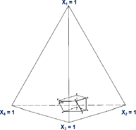
Table 6.10 – Lubricant Blending: Vertices of Formulation Region

6.10 Construction of Extreme Vertices Designs for Quadratic Formulation Models

As a general rule, when the components have lower and upper constraint, an extreme vertices design should be constructed such that the coefficients in the quadratic mixture model that is shown below can be estimated:

$$E(y)={\displaystyle \sum _{i=1}^q{b}_i{x}_i+{\displaystyle \sum {\displaystyle \sum _{1\le i<j}^q{b}_{ij}{x}_i{x}_j}}}$$

Those working with formulation systems have found that in the majority of cases the quadratic model gives a good fit to (or description of) the blending response surface. Special cubic terms are sometimes needed. In our experience it is rare that a full cubic model is required to provide an adequate fit to the response surface. An effective strategy, then, is to plan on the quadratic model being adequate, at least initially, per the principle of taking a sequential approach. In Chapter 10 we discuss more advanced model forms when quadratic or cubic models do not suffice.

The three- and four-component extreme vertices designs discussed previously were constructed assuming that the quadratic model would give an adequate fit to the response surface. In general, these designs contain the classes of points shown in Table 6.11.

Table 6.11 – Three- and Four-Component Formulations Experiments: Recommended Blends

Point Class	Three Components	Four or More Components
Vertices	X	X
Midpoints of Long Edges	X	X
Constraint Plane Centroids		X
Overall Centroid	X	X

Three-component designs are unique in that the constraint planes and edges are the same set of points. Hence, only the edge centroids (midpoints) are included in the three-component design described above.

Designs for five or more components are based on the same point classes as the four-component design--namely, vertices, edge centroids, constraint plane centroids, and the overall centroid. Unfortunately, the number of points in these classes can be quite large (100 or more for a five-component problem is not uncommon), and it becomes necessary to base the design on a subset of these points. Sophisticated computer algorithms such as those discussed in Chapters 7 and 8 are needed to select an optimum subset. Some alternative procedures that generate good (but not optimal) designs and that do not require these computer programs are also discussed in Chapters 7 and 8.

Replication and Assessing Model Lack of Fit

Another important consideration in constructing designs is the number of distinct blends and the amount of replication to be included in the design. The bare minimum design size is the number of points equal to the number of terms in the model. Such a design is often referred to as a saturated design and is not generally recommended. A general guideline is to select a design size that is 5 to 10 points more than the number of terms in the model. For example, in the case of four components, the quadratic model has ten coefficients; four linear blending terms, and six quadratic blending terms. Thus, the recommended design for a 10-term model would be 15 to 20 blends.

It is important to include some replicates in the design to estimate experimental variation (error), which is used to formally test the lack of fit of the model. An effective minimum is the “5+5” strategy; 5 blends more than the number of parameter in the model and 5 of the points in the design duplicated. Five degrees of freedom provides an F test for lack of fit that has adequate power.

As discussed in Chapter 4, a lack-of-fit test splits the residual variation into “pure error”, which is the variation among replicated points, and lack of fit, which represents variation between the model predictions and the actual values, or actual averages in the case of replicated points. The term pure error refers to the fact that this variation is not dependent on the model since it is just variation between replicated points, regardless of the model used. Conversely, the lack of fit is dependent on the model chosen. Therefore, if these two measures of variation are roughly equal, then the model appears to fit the data as well as could be expected, given the degree of error in replicates. However, if the lack-of-fit variation is much larger than the pure error, we have evidence of model inadequacy.

An F test is typically used to compare these measures of variation. The null hypothesis is that the population variances represented by these sample statistics are equal, but the alternative is that the lack-of-fit variance is larger. See Montgomery et al. (2012) for a more detailed discussion of lack-of-fit tests.

Fitting the four-component quadratic model to the results of 20 runs consisting of 15 blends plus repeats of 5 of the 15 distinct blends produces the analysis of variance (ANOVA) for lack of fit shown in Table 6.12. Note that the degrees of freedom for lack of fit and pure error sum to the overall error degrees of freedom

Table 6.12 – Example Four-Component Model: Lack-of-Fit ANOVA

Source of Variation	Degrees of Freedom	Mean Square	F-Ratio	Prob>F
Model	9
Lack of Fit	5	MS1	MS1/MS2	p
Pure Error	5	MS2
Error	10

A significant lack-of-fit F-ratio (e.g., p<0.05) indicates that the deviations between the model and the test results are statistically significant--i.e., we have statistical evidence of model inadequacy. Significant model lack of fit can be due to the need for a higher order model to fit the curvature in the data, or there may be some atypical (outlier) test results present in the data. A residual analysis will be helpful in understanding the source of the model lack of fit, as discussed in Chapter 4.

6.11 Designs for Formulation Systems with Multicomponent Constraints

Physical and economic considerations encountered in experimentation with formulations can impose multicomponent constraints on the region of feasible formulations. For example, in a plastic product formulation (Snee 1979), the liquid plasticizer content defined by the amounts of components 3, 4, and 5 was constrained to be between 25% and 35% of the total mixture. Here is an example:

0.25 < x₃ + x₄ + x₅ < 0.35.

In another situation, it might be desired that the ratio of components 1 and 4 be greater than 0.5,   x₁/x₄ > 0.50, which is equivalent to the linear constraint, 0 < x₁ – 0.5x₄.

The experimental region for an illustrative three component example defined by the following single component and multicomponent constraints is shown in Figure 6.15.

Variable	Lower Bound	Upper Bound
X1	0.10	0.50
X2	0.10	0.70
X3	0.00	0.70
85X1 + 90X2 + 100X3	90	95

The JMP commands that produce the six vertices of the region defined by the constraints are DOE ► Classical ► Mixture Design ► Extreme Vertices with Degree=1. The multiple component constraint is defined in the JMP Linear Constraints section as shown Figure 6.14.

Figure 6.14 – Multicomponent Example: Computation of Vertices – JMP Output

Figure 6.15 – Three-Component Example with Upper and Lower Bounds on the Components and Multiple Component Constraints

These constraints are all of the following general form:

a < a₁x₁ + a₂x₂ + ... + a_qx_q < b

In the form, the a_i’s are constants that are not all equal to one. The recommended approach to the design of formulation studies in the presence of multicomponent constraints is the same as that for single component constraints: a_i < x_i < b_i. The vertices of the experimental region are computed, and the design consists of a subset of the vertices and centroids of the region.

The CONSIM (CONstrained SIMplex) algorithm proposed by Snee (1979, 1981) can be used to compute the vertices.  The CONSIM algorithm will compute the vertices of an experimental region defined by both single component and multicomponent constraints such as those shown in Figure 6.15. The CONVERT, CONAEV, and MIXSOFT algorithms proposed by Piepel (1988, 1992) can also be used to compute the vertices of the experimental region. MIXSOFT software, which uses the CONVERT and CONAEV algorithms, is available from Piepel (1992). Computation of extreme vertices is also available in software systems such as JMP, Minitab, and Design Ease. All computations in this book were done using JMP 13.

Regions defined by single and/or multiple component constraints will often produce a large number of candidate vertices and centroids in cases where there are five or more components. When it is not practical to prepare and test all the candidate blends, we recommend that the experimental design selection algorithms discussed in Chapter 8 be used to select a subset of the vertices and centroids.

6.12 Sustained Release Tablet Formulation Study

Lewis et al. (1999) described a study that investigated the effects of four components on the performance of a sustained release tablet. Here are the four components studied and the associated upper and lower bounds:

Component	Lower Bound	Upper Bound
X1=Polymer	0.17	0.25
X2=Lactose	0.05	0.42
X3=Phosphate	0.05	0.47
X4=Cellulose	0.05	0.52

The uniqueness of the formulation was a hydrophilic cellulose polymer that swells in the presence of water and impedes the release of the active ingredient in the tablet. The study involved evaluating the effects of variations in the polymer levels and in the amounts of three diluents: lactose, phosphate, and cellulose.

The available region for experimentation that was defined by the four components has 12 vertices. It is shown in Figure 6.16, as adapted from Lewis et al. (1999). A computer algorithm was used to select the blends to be evaluated. Use of computer-aided design algorithms will be discussed in Chapter 8.

The resulting 17-point design is shown in Table 6.14 along with a critical response t50, which is the time in hours that it takes for 50% of the drug to dissolve. The goal is for t50 to be greater than 9.0 hours. The first 12 blends in Table 6.14 are the vertices of the region shown in Figure 6.16. The remaining five blends represent a subset of the centroids of the region.

Recalling that the goal is to find a formulation that has a t50 > 9.0, we examine the results in Table 6.14. We find that five blends have t50 > 9—namely, blends 1, 2, 6, 10, and 12. This gives us confidence that we can find a formulation that will meet the goals of the experiment.

Figure 6.16 – Sustained Release Tablet Experimental Region

Table 6.14 – Sustained Release Tablet Experiment: Design Blends

Blend	Polymer	Lactose	Phosphate	Cellulose	t50
1	0.17	0.05	0.26	0.52	9.56
2	0.25	0.05	0.18	0.52	12.05
3	0.17	0.42	0.05	0.36	6.19
4	0.25	0.42	0.05	0.28	8.09
5	0.17	0.05	0.47	0.31	8.76
6	0.25	0.05	0.47	0.23	11.51
7	0.17	0.42	0.36	0.05	6.75
8	0.25	0.42	0.28	0.05	8.56
9	0.17	0.26	0.05	0.52	6.08
10	0.25	0.18	0.05	0.52	9.71
11	0.17	0.31	0.47	0.05	6.18
12	0.25	0.23	0.47	0.05	11.84
13	0.21	0.05	0.22	0.52	8.51
14	0.21	0.42	0.05	0.32	6.96
15	0.21	0.27	0.47	0.05	7.39
16	0.21	0.32	0.05	0.42	6.57
17	0.21	0.24	0.26	0.29	8.83

An examination of the plots of t50 versus the component levels in Figure 6.17 shows that polymer and lactose appear to have the largest effects. Also, four of the five blends with t50 > 9 are at the high level of polymer.

The next step is to fit a model to the data and construct contour plots. The design was constructed to support the fitting of a 10-term quadratic model. The statistics for the fit of this model are shown in Table 6.15. The model fits the data well, showing an adjusted R² of 80%. Several of the quadratic terms involving the polymer component are large (t-ratios of approximately 2.0), and this is consistent with the polymer response curve shown in Figure 6.17. This indicates that curvilinear blending involving polymer is present. The model was fit using pseudo-components to reduce the effects of correlations among the model terms. This aspect of modeling--addressing correlations among the model terms--will be discussed further in Chapter 10.

Figure 6.17 – Sustained Release Tablet Study: Response (t50) vs Component Levels

Table 6.15 – Sustained Release Tablet Study:Quadratic Model - JMP Output

The contour plots for t50 as a function of cellulose, lactose, and phosphate at fixed polymer levels are shown in Figure 6.18. The response (t50) contours are shown at three levels of polymer: 17, 21, and 25% that appear top to bottom in Figure 6.18. The contours represent predicted values of t50 of 9.0 and higher. The figure was created in the same manner as Figure 6.12 above. We used the Contour Plot option in the JMP Mixture Profiler accessed by the following JMP commands: Analyze ► Fit Model ► (click Response Red Triangle) ► Factor Profiler ► Mixture Profiler Grid (click Mixture Profiler red triangle) ► Contour Grid.

Figure 6.18 – Sustained Release Tablet Experiment: Response Surface Contour Plots

In Figure 6.18 we see that as the level of polymer increases, the predicted value of t50 increases. We also see that the number of possible formulations of the three diluents that will meet the goal of t50 > 9.0 increases as the polymer level increases. In other words, the design space for the three diluents increases in size showing that there are more possible combinations of the three diluents to choose from and still meet the goal of t50 >9.

In general terms, the desirable region is at high polymer, low level of lactose, and equal proportions of phosphate and cellulose. Here are some possible formulations:

Candidate Formulation	Polymer	Lactose	Phosphate	Cellulose	Predicted t50
1	0.25	0.05	0.35	0.35	12.6
2	0.25	0.15	0.30	0.30	12.1
3	0.25	0.25	0.25	0.25	11.3
4	0.25	0.35	0.20	0.20	10.2

The final decision about which formulation to adopt will include other considerations as well, including material and manufacturing cost, ease of manufacture, and other properties of the formulation such as tablet hardness and friability (tendency of a pharmaceutical tablet to chip, crumble, or break).

6.13 Summary and Looking Forward

In this chapter we discussed how upper and lower bounds on the components affect the region of experimentation and how to construct formulation experiments in this situation. We also addressed the situation where, in addition to upper and lower bounds on the components, there may also be multiple component constraints that must be addressed. Fortunately, most of the same concepts, methods, and tools used when upper and lower bounds are involved apply when multiple component constraints must be addressed.  Our discussion included how to develop models for the data and how to interpret response surface contour plots of the predicted responses to select useful formulations.

We focused on three- and four-component systems to help clarify the issues involved, as these are easier to graph. In Chapter 8 we will discuss response surface experiments involving more components. But first we must discuss the design, analysis, and interpretation of screening experiments when the components have single and multiple component constraints. This will be the subject of Chapter 7.

6.14 References

Gorman, J. W. (1970) “Fitting Equations to Mixture Data with Restraints on Compositions.” Journal of Quality Technology, 2 (4), 186-194.

Hirata, M., K. Takayama and T. Nagai. (1992) “Formulation Optimization of Sustained-Release Tablet of Chlorpheniramine Maleate by Means of Extreme Vertices Design and Simultaneous Optimization Technique.” Chemical and Pharmaceutical Bulletin, 40 (3), 741-746.

Lewis, G. A., D. Mathieu and R. Phan-Tan-Luu. (1999) Pharmaceutical Experimental Design, Marcel Dekker, New York, NY.

McLean, R. A. and V. L. Anderson. (1966) “Extreme Vertices Design of Mixture Experiments.” Technometrics, 8 (3), 447-454.

Montgomery, D.C., Peck, E.A., and Vining, G.G. (2012) Introduction to Linear Regression Analysis, 5^th Edition, John Wiley & Sons, Hoboken, NJ.

Piepel, G. F. (1988) “Programs for Generating Extreme Vertices and Centroids of Linearly Constrained Experimental Regions.” Journal of Quality Technology, 20 (2), 125-139.

Piepel, G. F. (1992)  “MIXSOFT Version 2.0, Rev. 1, and MIXSOFT User’s Guide Version 2.06, MIXSOFT-Mixture Experiment Software.” Richland Washington, WA.

Snee, R. D. (1975) “Experimental Designs for Quadratic Models in Constrained Mixture Spaces.” Technometrics, 17 (2), 149-159.

Snee, R. D. (1979) “Experimental designs for mixture systems with multicomponent constraints.” Communications in Statistics, Theory and Methods, 8 (4), 303-326.

Snee, R. D.  (1981) “Developing Blending models for Gasoline and other Mixtures.” Technometrics, 23 (2), 119-130.