
Profiler Overview
Note: For details about the profilers in the Destructive Degradation platform, see the Destructive Degradation chapter in the Reliability and Survival Methods book.
The Profiler displays profile traces (see Figure 2.2) for each X variable. A profile trace is the predicted response as one variable is changed while the others are held constant at the current values. The Profiler recomputes the profiles and predicted responses (in real time) as you vary the value of an X variable.
• The vertical dotted line for each X variable shows its current value or current setting. If the variable is nominal, the x-axis identifies categories.
For each X variable, the value above the factor name is its current value. You change the current value by clicking in the graph or by dragging the dotted line where you want the new current value to be.
• The horizontal dotted line shows the current predicted value of each Y variable for the current values of the X variables.
• The black lines within the plots show how the predicted value changes when you change the current value of an individual X variable. In fitting platforms, the 95% confidence interval for the predicted values is shown by solid blue curves surrounding the prediction trace (for continuous variables) or the height of an error bar (for categorical variables). For continuous variables, the confidence interval region is shaded.
The Profiler is a way of changing one variable at a time and looking at the effect on the predicted response.
Figure 2.2 Illustration of Traces

The Profiler in some situations computes confidence intervals for each profiled column. If you have saved both a standard error formula and a prediction formula for the same column, the Profiler offers to use the standard errors to produce the confidence intervals rather than profiling them as a separate column.
Introduction to Profiling
It is easy to visualize a response surface with one input factor X and one output factor Y. It becomes harder as more factors and responses are added. The profilers in JMP provide a number of highly interactive cross-sectional views of any response surface.
Desirability profiling and optimization features are available to help find good factor settings and produce desirable responses. Most profilers also incorporate multithreading for faster computation. Simulation and defect profiling features are available for when you need to make responses that are robust and high-quality when the factors have variation.
Profiler Features in JMP
There are several profiler facilities in JMP, accessible from a number of fitting platforms and the main menu under Graph. They are used to profile data column formulas.
|
|
Description
|
Features
|
|
Profiler (or Prediction Profiler)
|
Shows vertical slices across each factor, holding other factors at current values
|
Desirability, Optimization, Simulator, Propagation of Error
|
|
Contour Profiler
|
Horizontal slices show contour lines for two factors at a time
|
Simulator
|
|
Surface Profiler
|
3-D plots of responses for 2 factors at a time, or a contour surface plot for 3 factors at a time
|
Surface Visualization
|
|
Mixture Profiler
|
A contour profiler for mixture factors
|
Ternary Plot and Contours
|
|
Custom Profiler
|
A non-graphical profiler and numerical optimizer
|
General Optimization, Simulator
|
|
Excel Profiler
|
Visualize models (or formulas) stored in Excel worksheets.
|
Profile using Excel Models
|
Profiler availability is shown in Table 2.2. The Custom Profiler is available only through the Graph menu. (Model Comparison does have Custom Profiler available.)
|
Location
|
Profiler
|
Contour Profiler
|
Surface Profiler
|
Mixture Profiler
|
|
Graph Menu (as a Platform)
|
Yes
|
Yes
|
Yes
|
Yes
|
|
Fit Model: Least Squares
|
Yes
|
Yes
|
Yes
|
Yes
|
|
Fit Model: Generalized Regression
|
Yes
|
|
|
|
|
Fit Model: Mixed Model
|
Yes
|
Yes
|
Yes
|
Yes
|
|
Fit Model: Logistic
|
Yes
|
|
|
|
|
Fit Model: Loglinear Variance
|
Yes
|
Yes
|
Yes
|
|
|
Fit Model: Generalized Linear Model
|
Yes
|
Yes
|
Yes
|
|
|
Fit Model: Partial Least Squares
|
Yes
|
|
|
|
|
Neural
|
Yes
|
Yes
|
Yes
|
|
|
Model Comparison
|
Yes
|
Yes
|
Yes
|
Yes
|
|
Nonlinear: Factors and Response
|
Yes
|
Yes
|
Yes
|
|
|
Nonlinear: Parameters and SSE
|
Yes
|
Yes
|
Yes
|
|
|
Nonlinear: Fit Curve
|
Yes
|
|
|
|
|
Gaussian Process
|
Yes
|
Yes
|
Yes
|
|
|
Partial Least Squares
|
Yes
|
|
|
|
|
Life Distribution
|
Yes
|
|
|
|
|
Fit Life by X
|
Yes
|
|
Yes
|
|
|
Recurrence Analysis
|
Yes
|
|
|
|
|
Choice
|
Yes
|
|
|
|
|
Custom Design Prediction Variance
|
Yes
|
|
Yes
|
|
|
Note: In this guide, we use the following terms interchangeably:
• factor, input variable, X column, independent variable, setting, term
• response, output variable, Y column, dependent variable, outcome
The Profiler (with a capital P) is one of several profilers (lowercase p). Sometimes, to distinguish the Profiler from other profilers, we call it the Prediction Profiler.
|
Profiler Launch Windows
When a profiler is invoked as a platform from the Graph menu, rather than through a fitting platform, you provide columns with formulas as the Y, Prediction Formula columns. These formulas could have been saved from the fitting platforms.
Figure 2.3 shows an example of most Profiler launch windows.
Figure 2.3 Profiler Launch Window

The columns referenced in the formulas become the X columns (unless the column is also a Y).
Y, Prediction Formula
The response columns containing formulas.
Noise Factors
Only used in special cases for modeling derivatives. For more information, about noise factors, see “Noise Factors”.
Expand Intermediate Formulas
Tells JMP that if an ingredient column to a formula is a column that itself has a formula, to substitute the inner formula, as long as it refers to other columns. To prevent an ingredient column from expanding, add an Other column property, name it Expand Formula, and assign a value of 0. For more information, see “Expand Intermediate Formulas”.
The Surface Plot platform is discussed in the Surface Plot chapter. The Surface Profiler is very similar to the Surface Plot platform, except Surface Plot has more modes of operation. Neither the Surface Plot platform nor the Surface Profiler have some of the capabilities common to other profilers.
Expand Intermediate Formulas
The Profiler launch window has an Expand Intermediate Formulas check box. When this is checked, when the formula is examined for profiling, if it references another column that has a formula containing references to other columns, then it substitutes that formula and profiles with respect to the end references—not the intermediate column references.
For example, when Fit Model fits a logistic regression for two levels (say A and B), the end formulas (Prob[A] and Prob[B]) are functions of the Lin[x] column, which itself is a function of another column x. If Expand Intermediate Formulas is selected, then when Prob[A] is profiled, it is with reference to x, not Lin[x].
In addition, using the Expand Intermediate Formulas check box enables the Save Expanded Formulas command in the platform red triangle menu. This creates a new column with a formula, which is the formula being profiled as a function of the end columns, not the intermediate columns.
Fit Group
For the REML and Stepwise personalities of the Fit Model platform, if models are fit to multiple Y’s, the results are combined into a Fit Group report. This enables the different Y’s to be profiled in the same Profiler. The Fit Group red triangle menu has options for launching the joint Profiler. Profilers for the individual Y’s can still be used in the respective Fit Model reports.
Fit Group reports are also created when a By variable is specified for a Stepwise analysis. This allows for the separate models to be profiled in the same Profiler.
The Fit Group scripting command can be used to fit models in different platforms, and have the individual models profiled in the Profiler. For more details, see the JMP Platforms chapter in the Scripting Guide.
Interpret the Profiles
The illustration in Figure 2.4 describes how to use the components of the Profiler. There are several important points to note when interpreting a prediction profile:
• The importance of a factor can be assessed to some extent by the steepness of the prediction trace. If the model has curvature terms (such as squared terms), then the traces might be curved.
• If you change the value of a factor, the prediction trace for that factor is not affected, but the prediction traces of all the other factors can change. The Y response line must cross the intersection points of the prediction traces with their current value lines.
Note: If there are interaction effects or cross-product effects in the model, the prediction traces can shift their slope and curvature as you change current values of other terms. That is what interaction is all about. If there are no interaction effects, the traces only change in height, not slope or shape.
Figure 2.4 Changing One Factor from 0 to 0.75

Prediction profiles are especially useful in multiple-response models to help judge that factor values can optimize a complex set of criteria.
Click a graph or drag the current value line right or left to change the factor’s current value. The response values change as shown by a horizontal reference line in the body of the graph. Double-click in an axis to bring up a window that changes its settings.
The Profiler as a Cross-Section
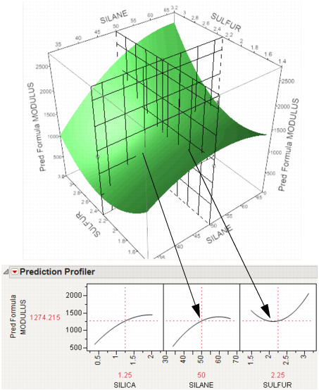
In the following example using Tiretread.jmp, look at the response surface of the expression for MODULUS as a function of SULFUR and SILANE (holding SILICA constant). Now look at how a grid that cuts across SILANE at the SULFUR value of 2.25. Note how the slice intersects the surface. If you transfer that down below, it becomes the profile for SILANE. Similarly, note the grid across SULFUR at the SILANE value of 50. The intersection when transferred down to the SULFUR graph becomes the profile for SULFUR.
Figure 2.5 Profiler as a Cross-Section
Now consider changing the current value of SULFUR from 2.25 to 1.5.
Figure 2.6 Profiler as a Cross-Section

In the Profiler, note the new value just moves along the same curve for SULFUR, the SULFUR curve itself does not change. But the profile for SILANE is now taken at a different cut for SULFUR. The profile for SILANE is also a little higher and reaches its peak in the different place, closer to the current SILANE value of 50.
Set or Lock Factor Values
If you ALT-click (Option-click on the Macintosh) in a graph, a window prompts you to enter specific settings for the factor.
Figure 2.7 Continuous Factor Settings Window

For continuous variables, you can specify:
Current Value
The value used to calculate displayed values in the profiler, equivalent to the red vertical line in the graph.
Minimum Setting
The minimum value of the factor’s axis.
Maximum Value
The maximum value of the factor’s axis.
Number of Plotted Points
Specifies the number of points used in plotting the factor’s prediction traces.
Show
Show or hide the factor in the profiler.
Lock Factor Setting
Locks the value of the factor at its current setting.
Profiler Platform Options
The red triangle menu on the Profiler title bar has the following options:
Profiler
Shows or hides the Profiler.
Contour Profiler
Shows or hides the Contour Profiler.
Custom Profiler
Shows or hides the Custom Profiler.
Surface Profiler
Shows or hides the Surface Profiler.
Mixture Profiler
Shows or hides the Mixture Profiler.
Save for Adobe Flash Platform (.SWF)
Enables you to save the Profiler (with reduced functionality) as an Adobe Flash file, which can be imported into presentation and web applications. An HTML page can be saved for viewing the Profiler in a browser. The Save for Adobe Flash platform (SWF) command is not available for categorical responses. For more information about this option, go to http://www.jmp.com/support/swfhelp/.
The Profiler accepts any JMP function, but the Flash Profiler only accepts the following functions: Add, Subtract, Multiply, Divide, Minus, Power, Root, Sqrt, Abs, Floor, Ceiling, Min, Max, Equal, Not Equal, Greater, Less, GreaterorEqual, LessorEqual, Or, And, Not, Exp, Log, Log10, Sine, Cosine, Tangent, SinH, CosH, TanH, ArcSine, ArcCosine, ArcTangent, ArcSineH, ArcCosH, ArcTanH, Squish, If, Match, Choose.
Note: Some platforms create column formulas that are not supported by the Save As Flash option.
Show Formulas
Opens a JSL window showing all formulas being profiled.
Formulas for OPTMODEL
Creates code for the OPTMODEL SAS procedure. Hold down CTRL and SHIFT and then select Formulas for OPTMODEL from the red triangle menu.
The following options are available in many platforms. See the JMP Reports chapter in the Using JMP book for more information.
Redo
Contains options that enable you to repeat or relaunch the analysis. In platforms that support the feature, the Automatic Recalc option immediately reflects the changes that you make to the data table in the corresponding report window.
Save Script
Contains options that enable you to save a script that reproduces the report to several destinations.
Common Profiler Topics
This section contains information on features that are common to more than one of the profiler platforms.
Linear Constraints
The Prediction Profiler, Custom Profiler, and Mixture Profiler can incorporate linear constraints into their operations. Linear constraints can be entered in two ways, described in the following sections.
Red Triangle Menu Item
To enter linear constraints via the red triangle menu, select Alter Linear Constraints from either the Prediction Profiler or Custom Profiler red triangle menu.
Choose Add Constraint from the resulting window, and enter the coefficients into the appropriate boxes. For example, to enter the constraint p1 + 2*p2 ≥ 0.9, enter the coefficients as shown in Figure 2.8. As shown, if you are profiling factors from a mixture design, the mixture constraint is present by default and cannot be modified.
Figure 2.8 Enter Coefficients

After you click OK, the Profiler updates the profile traces, and the constraint is incorporated into subsequent analyses and optimizations.
If you attempt to add a constraint for which there is no feasible solution, a message is written to the log and the constraint is not added. To delete a constraint, enter zeros for all the coefficients.
Constraints added in one profiler are not accessible by other profilers until saved. For example, if constraints are added under the Prediction Profiler, they are not accessible to the Custom Profiler. To use the constraint, you can either add it under the Custom Profiler red triangle menu, or use the Save Linear Constraints command described in the next section.
Constraint Table Property/Script
If you add constraints in one profiler and want to make them accessible by other profilers, use the Save Linear Constraints command, accessible through the platform red triangle menu. For example, if you created constraints in the Prediction Profiler, choose Save Linear Constraints under the Prediction Profiler red triangle menu. The Save Linear Constraints command creates or alters a Table Script called Constraint. An example of the Table Property is shown in Figure 2.9.
Figure 2.9 Constraint Table Script

The Constraint Table Property is a list of the constraints, and is editable. It is accessible to other profilers, and negates the need to enter the constraints in other profilers. To view or edit Constraint, right-click the red triangle menu and select Edit. The content of the constraint from Figure 2.8 is shown below in Figure 2.10.
Figure 2.10 Example Constraint

The Constraint Table Script can be created manually by choosing New Script from the red triangle menu beside a table name.
Note: When creating the Constraint Table Script manually, the spelling must be exactly “Constraint”. Also, the constraint variables are case sensitive and must match the column name. For example, in Figure 2.10, the constraint variables are p1 and p2, not P1 and P2.
The Constraint Table Script is also created when specifying linear constraints when designing an experiment.
The Alter Linear Constraints and Save Linear Constraints commands are not available in the Mixture Profiler. To incorporate linear constraints into the operations of the Mixture Profiler, the Constraint Table Script must be created by one of the methods discussed in this section.
Noise Factors
Note: Noise factor optimization is also available in the Prediction Profiler, Contour Profiler, Custom Profiler, and Mixture Profiler.
Robust process engineering enables you to produce acceptable products reliably, despite variation in the process variables. Even when your experiment has controllable factors, there is a certain amount of uncontrollable variation in the factors that affects the response. This is called transmitted variation. Factors with this variation are called noise factors. Some factors you cannot control at all, like environmental noise factors. The mean for some factors can be controlled, but not their standard deviation is not controllable. This is often the case for intermediate factors that are output from a different process or manufacturing step.
A good approach to making the process robust is to match the target at the flattest place of the noise response surface. Then, the noise has little influence on the process. Mathematically, this is the value where the first derivatives of each response with respect to each noise factor are zero. JMP computes the derivatives for you.
Figure 2.11 Noise Factor Example

Noise factors (robust process engineering) enables you to produce acceptable products reliably, despite variation in the process variables. Even when your experiment has controllable factors, there is a certain amount of uncontrollable variation in the factors that affects the response. This is called transmitted variation. Factors with this variation are called noise factors. You cannot control some factors, like environmental noise factors. The mean for some factors can be controlled, but their standard deviation is uncontrollable. This is often the case for intermediate factors that are output from a different process or manufacturing step.
A good approach to making the process robust is to match the target at the flattest place of the noise response surface. Then, the noise has little influence on the process. Mathematically, this is the value where the first derivatives of each response with respect to each noise factor are zero. JMP computes the derivatives for you.
To analyze a model with noise factors:
1. Fit the appropriate model (for example, using the Fit Model platform).
2. Save the model to the data table with the Save > Prediction Formula command.
3. Launch the Profiler (from the Graph menu).
4. Assign the prediction formula to the Y, Prediction Formula role and the noise factors to the Noise Factor role.
5. Click OK.
The resulting profiler shows response functions and their appropriate derivatives with respect to the noise factors, with the derivatives set to have maximum desirability at zero.
6. Select Optimization and Desirability > Maximize Desirability from the Profiler menu.
This finds the best settings of the factors, balanced with respect to minimizing transmitted variation from the noise factors.
..................Content has been hidden....................
You can't read the all page of ebook, please click here login for view all page.