
Data preprocessing is a crucial step for any data analysis problem. The model's accuracy depends mostly on the quality of the data. In general, any data preprocessing step involves data cleansing, transformations, identifying missing values, and how they should be treated. Only the preprocessed data can be fed into a machine-learning algorithm. In this section, we will focus mainly on data preprocessing techniques. These techniques include similarity measurements (such as Euclidean distance, Cosine distance, and Pearson coefficient) and dimensionality-reduction techniques, such as Principal component analysis (PCA), which are widely used in recommender systems. Apart from PCA, we have singular value decomposition (SVD), subset feature selection methods to reduce the dimensions of the dataset, but we limit our study to PCA.
As discussed in the previous chapter, every recommender system works on the concept of similarity between items or users. In this section, let's explore some similarity measures such as Euclidian distance, Cosine distance, and Pearson correlation.
The simplest technique for calculating the similarity between two items is by calculating its Euclidian distance. The Euclidean distance between two points/objects (point x and point y) in a dataset is defined by the following equation:
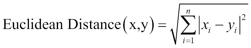
In this equation, (x, y) are two consecutive data points, and n is the number of attributes for the dataset.
R script to calculate the Euclidean distance is as follows:
x1 <- rnorm(30)
x2 <- rnorm(30)
Euc_dist = dist(rbind(x1,x2) ,method="euclidean")
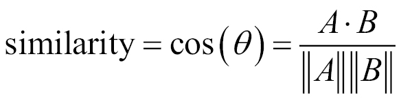
Cosine similarity is a measure of similarity between two vectors of an inner product space that measures the cosine of the angle between them. Cosine similarity is given by this equation:
R script to calculate the cosine distance is as follows:
vec1 = c( 1, 1, 1, 0, 0, 0, 0, 0, 0, 0, 0, 0 )
vec2 = c( 0, 0, 1, 1, 1, 1, 1, 0, 1, 0, 0, 0 )
library(lsa)
cosine(vec1,vec2)
In this equation, x is the matrix containing all variables in a dataset. The cosine function is available in the lsa package.
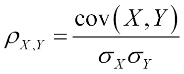
Similarity between two products can also be given by the correlation existing between their variables. Pearson's correlation coefficient is a popular correlation coefficient calculated between two variables as the covariance of the two variables divided by the product of their standard deviations. This is given by ƿ (rho):
R script is given by these lines of code:
Coef = cor(mtcars, method="pearson")
where mtcars is the dataset
Empirical studies showed that Pearson coefficient outperformed other similarity measures for user-based collaborative filtering recommender systems. The studies also show that Cosine similarity consistently performs well in item-based collaborative filtering.
One of the most commonly faced problems while building recommender systems is high-dimensional and sparse data. At many times, we face a situation where we have a large set of features and fewer data points. In such situations, when we fit a model to the dataset, the predictive power of the model will be lower. This scenario is often termed as the curse of dimensionality. In general, adding more data points or decreasing the feature space, also known as dimensionality reduction, often reduces the effects of the curse of dimensionality. In this chapter, we will discuss PCA, a popular dimensionality reduction technique to reduce the effects of the curse of dimensionality.
Principal component analysis is a classical statistical technique for dimensionality reduction. The PCA algorithm transforms the data with high-dimensional space to a space with fewer dimensions. The algorithm linearly transforms m-dimensional input space to n-dimensional (n<m) output space, with the objective to minimize the amount of information/variance lost by discarding (m-n) dimensions. PCA allows us to discard the variables/features that have less variance.
Technically speaking, PCA uses orthogonal projection of highly correlated variables to a set of values of linearly uncorrelated variables called principal components. The number of principal components is less than or equal to the number of original variables. This linear transformation is defined in such a way that the first principal component has the largest possible variance. It accounts for as much of the variability in the data as possible by considering highly correlated features. Each succeeding component in turn has the highest variance using the features that are less correlated with the first principal component and that are orthogonal to the preceding component.
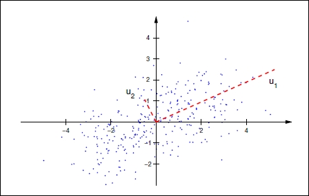
Let's understand this in simple terms. Assume we have three dimensional data space with two features more correlated with each other than with the third. We now want to reduce the data to two-dimensional space using PCA. The first principal component is created in such a way that it explains maximum variance using the two correlated variables along the data. In the following graph, the first principal component (bigger line) is along the data explaining most variance. To choose the second principal component, we need to choose another line that has the highest variance, is uncorrelated, and is orthogonal to the first principal component. The implementation and technical details of PCA are beyond the scope of this book, so we will discuss how it is used in R.
We will illustrate PCA using the USArrests dataset. The USArrests dataset contains crime-related statistics, such as Assault, Murder, Rape, and UrbanPop per 100,000 residents in 50 states in the US:
#PCA
data(USArrests)
head(states)
[1] "Alabama"    "Alaska"     "Arizona"    "Arkansas"   "California" "Colorado"

names(USArrests)
[1] "Murder"   "Assault"  "UrbanPop" "Rape"

#let us use apply() to the USArrests dataset row wise to calculate the variance to see how each variable is varying
apply(USArrests , 2, var)

Murder    Assault   UrbanPop       Rape
  18.97047 6945.16571  209.51878   87.72916
#We observe that Assault has the most variance. It is important to note at this point that

#Scaling the features is a very step while applying PCA.

#Applying PCA after scaling the feature as below
pca =prcomp(USArrests , scale =TRUE)

pca
Standard deviations:
[1] 1.5748783 0.9948694 0.5971291 0.4164494
Rotation:
                PC1        PC2        PC3         PC4
Murder   -0.5358995  0.4181809 -0.3412327  0.64922780
Assault  -0.5831836  0.1879856 -0.2681484 -0.74340748
UrbanPop -0.2781909 -0.8728062 -0.3780158  0.13387773
Rape     -0.5434321 -0.1673186  0.8177779  0.08902432

#Now lets us understand the components of pca output.

names(pca)
[1] "sdev"     "rotation" "center"   "scale"    "x"

#Pca$rotation  contains the principal component loadings matrix which explains

#proportion of each variable along each principal component.

#now let us learn interpreting the results of pca using biplot graph. Biplot is used to how the proportions of each variable along the two principal components.

#below code changes the directions of the biplot, if we donot include the below two lines the plot will be mirror image to the below one.
pca$rotation=-pca$rotation
pca$x=-pca$x
biplot (pca , scale =0)
The output of the preceding code is as follows:
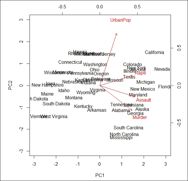
In the preceding image, known as a biplot, we can see the two principal components (PC1 and PC2) of the USArrests dataset. The red arrows represent the loading vectors, which represent how the feature space varies along the principal component vectors.
From the plot, we can see that the first principal component vector, PC1, more or less places equal weight on three features: Rape, Assault, and Murder. This means that these three features are more correlated with each other than the UrbanPop feature. In the second principal component, PC2 places more weight on UrbanPop than the remaining 3 features are less correlated with them.