In the previous sections, we have seen various data-mining techniques used in recommender systems. In this section, you will learn how to evaluate models built using data-mining techniques. The ultimate goal for any data analytics model is to perform well on future data. This objective could be achieved only if we build a model that is efficient and robust during the development stage.

While evaluating any model, the most important things we need to consider are as follows:

Under fitting, also known as bias, is a scenario when the model doesn't even perform well on training data. This means that we fit a less robust model to the data. For example, say the data is distributed non-linearly and we are fitting the data with a linear model. From the following image, we see that data is non-linearly distributed. Assume that we have fitted a linear model (orange line). In this case, during the model building stage itself, the predictive power will be low.

Over fitting is a scenario when the model performs well on training data, but does really bad on test data. This scenario arises when the model memorizes the data pattern rather than learning from data. For example, say the data is distributed in a non-linear pattern, and we have fitted a complex model, shown using the green line. In this case, we observe that the model is fitted very close to the data distribution, taking care of all the ups and downs. In this case, the model is most likely to fail on previously unseen data.

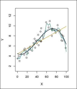
The preceding image shows simple, complex, and appropriate fitted models' training data. The green fit represents overfitting, the orange line represents underfitting, the black and blue lines represent the appropriate model, which is a trade-off between underfit and overfit.

Any fitted model is evaluated to avoid previously mentioned scenarios using cross validation, regularization, pruning, model comparisons, ROC curves, confusion matrices, and so on .

Cross validation: This is a very popular technique for model evaluation for almost all models. In this technique, we divide the data into two datasets: a training dataset and a test dataset. The model is built using the training dataset and evaluated using the test dataset. This process is repeated many times. The test errors are calculated for every iteration. The averaged test error is calculated to generalize the model accuracy at the end of all the iterations.

Regularization: In this technique, the data variables are penalized to reduce the complexity of the model with the objective to minimize the cost function. There are two most popular regularization techniques: ridge regression and lasso regression. In both techniques, we try to reduce the variable co-efficient to zero. Thus, a smaller number of variables will fit the data optimally.

Confusion matrix: This technique is popularly used in evaluating a classification model. We build a confusion matrix using the results of the model. We calculate precision and recall/sensitivity/specificity to evaluate the model.

Precision: This is the probability whether the truly classified records are relevant.

Recall/Sensitivity: This is the probability whether the relevant records are truly classified.

Specificity: Also known as true negative rate, this is the proportion of truly classified wrong records.

A confusion matrix shown in the following image is constructed using the results of classification models discussed in the previous section:

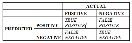
Let's understand the confusion matrix:

TRUE POSITVE (TP): This is a count of all the responses where the actual response is negative and the model predicted is positive

FALSE POSITIVE (FP): This is a count of all the responses where the actual response is negative, but the model predicted is positive. It is, in general, a FALSE ALARM.

FALSE NEGATIVE (FN): This is a count of all the responses where the actual response is positive, but the model predicted is negative. It is, in general, A MISS.

TRUE NEGATIVE (TN): This is a count of all the responses where the actual response is negative, and the model predicted is negative.

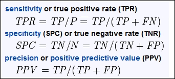
Mathematically, precision and recall/specificity is calculated as follows:

Model comparison: A classification problem can be solved using one or more statistical models. For example, a classification problem can be solved using logistic regression, a decision tree, ensemble methods, and SVM. How do you choose which model fits the data well? A number of approaches are available for a suitable model selection, such as Akaike information criteria (AIC), Bayesian information criteria (BIC), and Adjusted R^2, Cᵨ. For each model, AIC / BIC / Adjusted R^2 is calculated. The model with least of these values is selected as the best model.