Like many other R packages, recommenderlab contains some datasets that can be used to play around with the functions:

data_package <- data(package = "recommenderlab")
data_package$results[, "Item"]

data(MovieLense)
MovieLense
## 943 x 1664 rating matrix of class 'realRatingMatrix' with 99392 ratings.

In this section, we will explore MovieLense in detail:

class(MovieLense)
## [1] "realRatingMatrix"
## attr(,"package")
## [1] "recommenderlab"

The realRatingMatrix class is defined by recommenderlab, and ojectsojectsb contains sparse rating matrices. Let's take a look at the methods that we can apply on the objects of this class:

methods(class = class(MovieLense))

Some methods that are applicable to matrices have been redefined in a more optimized way. For instance, we can use dim to extract the number of rows and columns, and colSums to compute the sum of each column. In addition, there are new methods that are specific for recommendation systems.

Usually, rating matrices are sparse matrices. For this reason, the realRatingMatrix class supports a compact storage of sparse matrices. Let's compare the size of MovieLense with the corresponding R matrix:

object.size(MovieLense)
## 1388448 bytes
object.size(as(MovieLense, "matrix"))
## 12740464 bytes

We can compute how many times the recommenderlab matrix is more compact:

object.size(as(MovieLense, "matrix")) / object.size(MovieLense)
## 9.17604692433566 bytes

As expected, MovieLense occupies much less space than the equivalent standard R matrix. The rate is about 1:9, and the reason is the sparsity of MovieLense. A standard R matrix object stores all the missing values as 0s, so it stores 15 times more cells.

Collaborative filtering algorithms are based on measuring the similarity between users or between items. For this purpose, recommenderlab contains the similarity function. The supported methods to compute similarities are cosine, pearson, and jaccard.

For instance, we might want to determine how similar the first five users are with each other. Let's compute this using the cosine distance:

similarity_users <- similarity(MovieLense[1:4, ], method = "cosine", which = "users")

The similarity_users object contains all the dissimilarities. Let's explore it:

class(similarity_users)
## [1] "dist"

As expected, similarity_users is an object containing distances. Since dist is a base R class, we can use it in different ways. For instance, we could use hclust to build a hierarchic clustering model.

We can also convert similarity_users into a matrix and visualize it:

as.matrix(similarity_users)

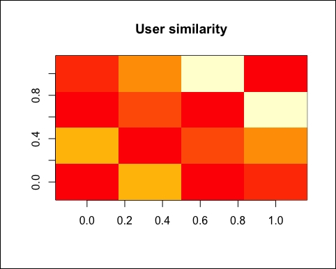
Using image, we can visualize the matrix. Each row and each column corresponds to a user, and each cell corresponds to the similarity between two users:

image(as.matrix(similarity_users), main = "User similarity")

The more red the cell is, the more similar two users are. Note that the diagonal is red, since it's comparing each user with itself:

Using the same approach, we can compute and visualize the similarity between the first four items:

similarity_items <- similarity(MovieLense[, 1:4], method = "cosine", which = "items")
as.matrix(similarity_items)

The table continues as follows:

Similar to the preceding screenshot, we can visualize the matrix using this image:

image(as.matrix(similarity_items), main = "Item similarity")

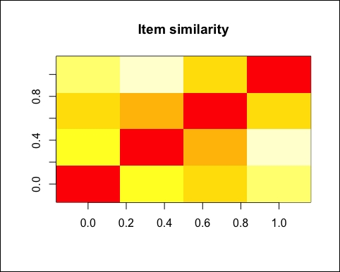
The similarity is the base of collaborative filtering models.

The recommenderlab package contains some options for the recommendation algorithm. We can display the model applicable to the realRatingMatrix objects using recommenderRegistry$get_entries:

recommender_models <- recommenderRegistry$get_entries(dataType = "realRatingMatrix")

The recommender_models object contains some information about the models. First, let's see which models we have:

names(recommender_models)

Let's take a look at their descriptions:

lapply(recommender_models, "[[", "description")
## $IBCF_realRatingMatrix
## [1] "Recommender based on item-based collaborative filtering (real data)."
##
## $PCA_realRatingMatrix
## [1] "Recommender based on PCA approximation (real data)."
##
## $POPULAR_realRatingMatrix## [1] "Recommender based on item popularity (real data)."
##
## $RANDOM_realRatingMatrix
## [1] "Produce random recommendations (real ratings)."
##
## $SVD_realRatingMatrix
## [1] "Recommender based on SVD approximation (real data)."
##
## $UBCF_realRatingMatrix
## [1] "Recommender based on user-based collaborative filtering (real data)."

Out of them, we will use IBCF and UBCF.

The recommender_models object also contains some other information, such as its parameters:

recommender_models$IBCF_realRatingMatrix$parameters

For a more detailed description of the package and some use cases, you can take a look at the package vignette. You can find all the material by typing help(package = "recommenderlab").

The recommenderlab package is a good and flexible package to perform recommendation. If we combine its models with other R tools, we will have a powerful framework to explore the data and build recommendation models.

In the next section, we will explore a dataset of recommenderlab using some of its tools.