The data is about Microsoft users visiting a website during one week. For each user, the data displays which areas the users visited. For the sake of simplicity, from now on we will refer to the website areas with the term "items".

There are 5,000 users and they are represented by sequential numbers between 10,001 and 15,000. Items are represented by numbers between 1,000 and 1,297, even if they are less than 298.

The dataset is an unstructured text file. Each record contains a number of fields between 2 and 6. The first field is a letter defining what the record contains. There are three main types of records, which are as follows:

Each case record is followed by one or more votes, and there is just one case for each user.

Our target is to recommend each user to explore some areas of the website that they haven't explored yet.

This section will show you how to import data. First, let's load the packages that we will use:

library("data.table")
library("ggplot2")
library("recommenderlab")
library("countrycode")

The preceding code is explained in the following points:

Then, let's load the table into memory. If the text file is already in our working directory, it's enough to define its name. Otherwise, we need to define its full path:

file_in <- "anonymous-msweb.test.txt"

The rows contain different numbers of columns, which means that the data is unstructured. However, there are at most six columns, so we can load the file into a table using read.csv. The rows with fewer than six fields will have just empty values:

table_in <- read.csv(file_in, header = FALSE)
head(table_in)

The first two columns contain the user IDs and their purchases. We can just drop the other columns:

table_users <- table_in[, 1:2]

In order to process the data more easily, we can convert it into a data table, using this command:

table_users <- data.table(table_users)

The columns are as follows:

We can assign the column names and select the rows containing either users or items:

setnames(table_users, 1:2, c("category", "value"))
table_users <- table_users[category %in% c("C", "V")]
head(table_users)

The table_users object contains structured data, which is our starting point to define a rating matrix.

Our target is to define a table having a row for each item and a column for each purchase. For each user, table_users contains its ID and purchases in separate rows. In each block or rows, the first column contains the user ID and the other contains the item IDs.

You can use the following steps to define a rating matrix:

In order to reshape the table, the first step is to define a field called chunk_user containing an incremental number for each user. The category == "C" condition is true for the user rows, which are the first rows of the chunks. Using cumsum, we are incrementing the index of 1 whenever there is a row with a new user:

table_users[, chunk_user := cumsum(category == "C")]
head(table_users)

The next step is to define a table in which rows correspond to the purchases. We need a column with the user ID and a column with the item ID. The new table is called table_long, because it's in a long format:

table_long <- table_users[, list(user = value[1], item = value[-1]), by = "chunk_user"]
head(table_long)

Now, we can define a table having a row for each user and a column for each item. The values are equal to 1 if the item has been purchased, and 0 otherwise. We can build the table using the reshape function. Its inputs are as follows:

After defining the column value equal to 1, we can build table_wide using reshape:

table_long[, value := 1]
table_wide <- reshape(data = table_long,direction = "wide",idvar = "user",timevar = "item",v.names = "value")
head(table_wide[, 1:5, with = FALSE])

In order to build the rating matrix, we need to keep only the columns containing ratings. In addition, the user name will be the matrix row names, so we need to store them in the vector_users vector:

vector_users <- table_wide[, user]
table_wide[, user := NULL]
table_wide[, chunk_user := NULL]

In order to have the column names equal to the item names, we need from the value prefix. For this purpose, we can use the substring function:

setnames(x = table_wide,old = names(table_wide),new = substring(names(table_wide), 7))

We need to store the rating matrix within a recommenderlab object. For this purpose, we need to convert table_wide in a matrix first. In addition, we need to set the row names equal to the user names:

matrix_wide <- as.matrix(table_wide)rownames(matrix_wide) <- vector_users
head(matrix_wide[, 1:6])

The last step is coercing matrix_wide into a binary rating matrix using as, in the following way:

matrix_wide[is.na(matrix_wide)] <- 0
ratings_matrix <- as(matrix_wide, "binaryRatingMatrix")
ratings_matrix
## 5000 x 236 rating matrix of class binaryRatingMatrix with 15191 ratings.

Let's take a look at the matrix using image:

image(ratings_matrix[1:50, 1:50], main = "Binary rating matrix")

The following image shows the binary rating matrix:

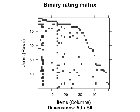
As expected, the matrix is sparse. We can also visualize the distributions of the number of users purchasing an item:

n_users <- colCounts(ratings_matrix)
qplot(n_users) + stat_bin(binwidth = 100) + ggtitle("Distribution of the number of users")

The following image displays the distribution of the number of users:

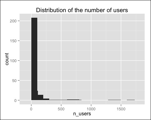
There are some outliers, that is, items purchased by many users. Let's visualize the distribution excluding them:

qplot(n_users[n_users < 100]) + stat_bin(binwidth = 10) + ggtitle("Distribution of the number of users")

The following image displays the distribution of the numbers of users:

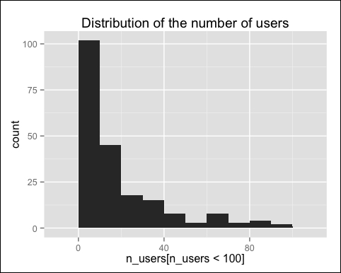
There are many items that have been purchased by a few users only, and we won't recommend them. Since they increase the computational time, we can just remove them by defining a minimum number of purchases, for example, 5:

ratings_matrix <- ratings_matrix[, colCounts(ratings_matrix) >= 5]
ratings_matrix
## 5000 x 166 rating matrix of class 'binaryRatingMatrix' with 15043 ratings.

Now, we have 166 items, compared to the initial 236. As regards users, we want to recommend items to everyone. However, there might be users that have purchased only items that we removed. Let's check it:

sum(rowCounts(ratings_matrix) == 0)
## _15_

There are 15 users with no purchases. These purchases should be removed. In addition, users who have purchased just a few items are difficult to deal with. Therefore, we only keep users that have purchased at least five items:

ratings_matrix <- ratings_matrix[rowCounts(ratings_matrix) >= 5, ]
ratings_matrix
## 959 x 166 rating matrix of class 'binaryRatingMatrix' with 6816 ratings

The table_in raw data contains some records starting with A, and they display some information about the items. In order to extract these records, we can convert table_in into a data table and extract the rows having A in the first column:

table_in <- data.table(table_in)
table_items <- table_in[V1 == "A"]
head(table_items)

The relevant columns are:

In order to have a more clear table, we can extract and rename them. In addition, we can sort the table by item ID:

table_items <- table_items[, c(2, 4, 5), with = FALSE]
setnames(table_items, 1:3, c("id", "description", "url"))
table_items <- table_items[order(id)]
head(table_items)

We need to identify one or more features describing the items. If we look at the table, we can identify two categories of web pages:

We can identify the records containing a geographic location, and consider the remaining as products. For this purpose, we can start defining the field category that, at the moment, is equal to product for all the records:

table_items[, category := "product"]

The country code package provides us with the countrycode_data object that contains most of the country names. We can define the name_countries vector that contains the names of countries and geographic locations. Then, we can categorize as region all the records whose description is in name_countries:

name_countries <- c(countrycode_data$country.name, "Taiwan", "UK", "Russia", "Venezuela", "Slovenija", "Caribbean", "Netherlands (Holland)", "Europe", "Central America", "MS North Africa")
table_items[description %in% name_countries, category := "region"]

There are other records containing the word region. We can identify them through a regular expression using grepl:

table_items[grepl("Region", description), category := "region"]
head(table_items)

Let's take a look at the result and find out the number of items we have for each category:

table_items[, list(n_items = .N), by = category]

About 80 percent of the web pages are products, and the remaining 20 percent are regions.

We are now ready to build recommendation models.