This section will show you how to define a function that:

The inputs of our function are as follows:

Let's define the function arguments. You can find the description of each argument as a comment next to its name:

evaluateModel <- function (
  # data inputs
  ratings_matrix, # rating matrix
  table_items, # item description table
  # K-fold parameters
  n_fold = 10, # number of folds
  items_to_keep = 4, # number of items to keep in the test set
  # model parameters
  number_neighbors = 30, # number of nearest neighbors
  weight_description = 0.2, # weight to the item description-based distance
  items_to_recommend = 10 # number of items to recommend
){
  # build and evaluate the model
}

Now, we can walk through the function body step by step. For a more detailed explanation, see the previous section and Chapter 4, Evaluating the Recommender Systems:

You can find a detailed description of the indices in Chapter 4, Evaluating the Recommender Systems.

In this section, we defined a function evaluating our model with given settings. This function will help us with parameter optimization.

Starting with our evaluateModel() function, we can optimize the model parameters. In this section, we will optimize these parameters:

Although we could optimize other parameters, we will just leave them to their defaults, for the sake of simplicity.

Our recommender model combines IBCF with the item descriptions. Therefore, it's a good practice to optimize IBCF first, that is, the number_neighbors parameter.

First, we have to decide which values we want to test. We take account of k, that is, at most, half of the items, that is, about 80. On the other hand, we exclude values that are smaller than 4, since the algorithm would be too unstable. Setting a granularity of 2, we can generate a vector with the values to test:

nn_to_test <- seq(4, 80, by = 2)

Now, we can measure the performance depending on number_neighbors. Since we are optimizing the IBCF part only, we will set weight_description = 0. Using lapply, we can build a list of elements that contain the performance for each value of nn_to_test:

list_performance <- lapply(
  X = nn_to_test,
  FUN = function(nn){
    evaluateModel(ratings_matrix = ratings_matrix, table_items = table_items, number_neighbors = nn, weight_description = 0)
  })

Let's take a look at the first element of the list:

list_performance[[1]]

The first element contains all the performance metrics. In order to evaluate our model, we can use the precision and recall. See Chapter 4, Evaluating the Recommender Systems for more information.

We can extract a vector of precisions (or recalls) using sapply:

sapply(list_performance, "[[", "precision")^t

0.1663, 0.1769, 0.1769, 0.175, 0.174, 0.1808, 0.176, 0.1779, 0.1788, 0.1788, 0.1808, 0.1817, 0.1817, 0.1837, 0.1846, 0.1837, 0.1827, 0.1817, 0.1827, 0.1827, 0.1817, 0.1808, 0.1817, 0.1808, 0.1808, 0.1827, 0.1827, 0.1837, 0.1827, 0.1808, 0.1798, 0.1798, 0.1798, 0.1798, 0.1798, 0.1798, 0.1788, 0.1788 and 0.1788

In order to analyze the output, we can define a table whose columns are nn_to_test, precisions, and recalls:

table_performance <- data.table(
  nn = nn_to_test, precision = sapply(list_performance, "[[", "precision"), recall = sapply(list_performance, "[[", "recall")
)

In addition, we can define a performance index that we will optimize. The performance index can be a weighted average between the precision and the recall. The weights depend on the use case, so we can just leave them to 50 percent:

weight_precision <- 0.5
table_performance[
    performance := precision * weight_precision + recall * (1 - weight_precision)]
head(table_performance)

The precision is the percentage of recommended items that have been purchased, and the recall is the percentage of purchased items that have been recommended.

The table_performance table contains all the evaluation metrics. Starting with it, we can build charts that help us identify the optimal nn.

Before building the charts, let's define the convertIntoPercent() function that we will use within the ggplot2 functions:

convertIntoPercent <- function(x){
  paste0(round(x * 100), "%")
}

We are ready to build the charts. The first chart is about the precision based on nn. We can build it using these functions:

The following command consists of the preceding points:

  qplot(table_performance[, nn], table_performance[, precision]) + geom_smooth() + scale_y_continuous(labels = convertIntoPercent)

The following image is the output of the preceding code:

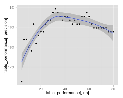
The smoothed line grows until the global maximum, which is around nn = 35, slowly decreases. This index expresses the percentage of recommendations that have been successful, so it's useful when there are high costs associated with advertising.

Let's take a look at the recall, using the same commands:

  qplot(table_performance[, nn], table_performance[, recall]) + geom_smooth() + scale_y_continuous(labels = convertIntoPercent)

The following image is the output of the preceding screenshot:

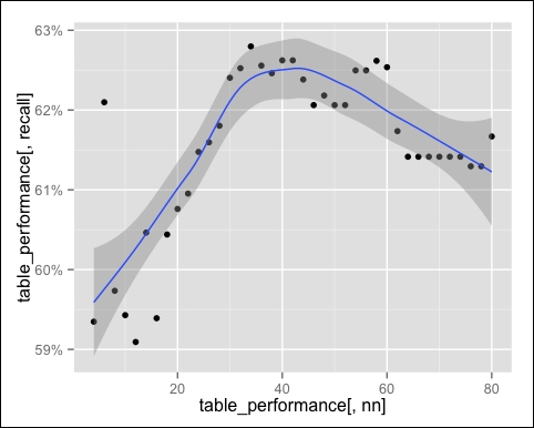
The maximum recall is around nn = 40. This index expresses the percentage of purchases that we recommended, so it's useful if we want to be sure to predict most of the purchases.

The performance takes account of the precision and the recall at the same time. Let's take a look at it:

  qplot(table_performance[, nn], table_performance[, performance]) + geom_smooth() + scale_y_continuous(labels = convertIntoPercent)

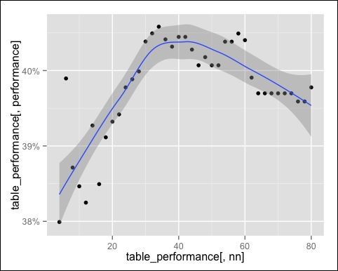
The optimal performances are between 30 and 45. We can identify the best nn using which.max:

row_best <- which.max(table_performance$performance)
number_neighbors_opt <- table_performance[row_best, nn]
number_neighbors_opt
## _34_

The optimal value is 34. We optimized the IBCF parameter, and the next step is determining the weight of the item description component. First, let's define the weights to try. The possible weights range between 0 and 1, and we just need to set the granularity, for instance, 0.05:

wd_to_try <- seq(0, 1, by = 0.05)

Using lapply, we can test the recommender based on the weight:

list_performance <- lapply(
  X = wd_to_try, FUN = function(wd){
    evaluateModel(ratings_matrix = ratings_matrix, table_items = table_items, number_neighbors = number_neighbors_opt, weight_description = wd) })

Just like we did earlier, we can build a table containing precisions, recalls, and performances:

table_performance <- data.table(
  wd = wd_to_try, precision = sapply(list_performance, "[[", "precision"), recall = sapply(list_performance, "[[", "recall")
)
table_performance[
    performance := precision * weight_precision + recall * (1 - weight_precision)]

Now, we can visualize the performance based on the weight through a chart:

  qplot(table_performance[, wd], table_performance[, performance]) + geom_smooth() + scale_y_continuous(labels = convertIntoPercent)

The following image is the output of the preceding command:

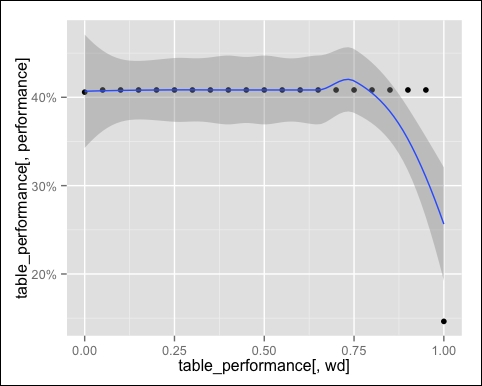
The performance is the same for each point, with the exception of the extremes. Therefore, the smoothing line is not useful.

We have the best performance that takes account of both ratings and descriptions. The extreme 0.00 corresponds to pure IBCF, and it performs slightly worse than the hybrid. The model in the extreme 1.00 is based on the item description only, and that's why it performs so badly.

The reason why the performance doesn't change much is that the item description is based on a binary feature only. If we add other features, we will see a greater impact.

This section showed you how to optimize our recommendation algorithm on the basis of two parameters. A next step could be optimizing on the basis of the remaining IBCF parameters and improving the item description.