
This chapter will introduce you to the underlying data structure of tables in Cassandra. Let's set some development rules of thumb before we dive into CQL. With CQL 3, Cassandra development team has done a commendable job of almost entirely eliminating any chance of using an antipattern, and at the same time bringing an interface that is SQL people friendly.
If you are a developer, this is probably the most important chapter for you. You will get a sense of things that are possible and not possible when working with Cassandra. You may also want to refer Chapter 8, Integration with Hadoop, to understand how to use Cassandra with various big data technologies such as the Hadoop ecosystem and Spark/Shark.
When dealing with Cassandra, keep the following things in mind:
- Denormalize, denormalize, and denormalize: Forget about old school 3NF in Cassandra; the fewer the network trips, the better the performance. Denormalize wherever you can for quicker retrieval and let the application logic handle the responsibility of reliably updating all the redundancies.
- Rows are gigantic and sorted: The giga-sized rows (a row can accommodate 2 billion cells per partition) can be used to store sortable and sliceable columns. Need to sort comments by timestamp? Need to sort bids by quoted price? Put in a column with the appropriate comparator (you can always write your own comparator).
- One row, one machine: Each row stays on one machine. Rows are not sharded across nodes. So beware of this. A high-demand row may create a hotspot.
- From query to model: Unlike RDBMS, where you model most of the tables with entities in the application and then run analytical queries to get data out of it, Cassandra has no such provision. So you may need to denormalize your model in such a way that all your queries stay limited to a bunch of simple commands such as
get,slice,count,multi_get, and some simple indexed searches.
From Version 1.2 onwards, Cassandra has CQL as its primary way to access and alter the database. CQL is an abstraction layer that makes you feel like you are working with RDBMS, but the underlying data model does not support all the features that a traditional database or SQL provides. There is no group by, no relational integrity, foreign key constraints, and no join. There is some support for order, distinct, and triggers. There are things such as time to live (TTL) and write time functions. So Cassandra, like most of the NoSQL databases, is generally less featured compared to the number of features traditional databases provide.
Cassandra is designed for extremely high-read and high-write speed and horizontal scalability. Without some of the analytical features of traditional systems, developers need to work around Cassandra's shortcomings by planning ahead. In the Cassandra community, it is generally referred to as modeling the database based on what queries you will run in future. Let's take an example. If you have a people database and you wanted to draw a bar chart that shows the number of people from different cities, in Cassandra, you cannot just run the select count(*), city from people group by city statement. Instead, you will have to create a different table that has city as its primary key and a counter column that holds the number of records of persons. Every time a people record is added or removed, you increase or decrease the counter for the specific city. Understanding underlying the data structure can help you rationalize why Cassandra can or cannot do some things.
If you remove all the complexity, the data in Cassandra is stored in a nested hash map– a hash map containing another hash map. Realistically speaking, it is a distributed, nested, sorted hash map where the outer sorted hash map is distributed across the machines and the inner one stays on one machine. The following figure shows the Cassandra data model:
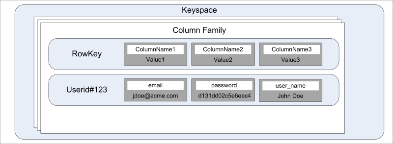
Cassandra has two ways of viewing its data: one is viewing data as maps within a map, the other is viewing it as a table. The former is the old way, and more closer to actually how the data is stored; and the latter is the new way, the way CQL represents the data. In this section, since we are trying to understand how the data is stored in Cassandra, we will go the old way. Then in the next section, we will see how this maps to CQL.
At the heart of Cassandra lies two structures: column family and cell. There is a container entity for these entities called keyspace.
Note
Previously, we used to call a cell a column. From Cassandra 1.2 onward, the nomenclature has been changed a bit to avoid confusion with columns as defined in CQL3. Columns in CQL3 are more in line with columns in the traditional database. "Column family" is the old name for a table. There is still a slight difference between the column family and table, but for the most part, we can use them interchangeably.
A cell is the smallest unit of the Cassandra data model. Cells are contained within a column family. A cell is essentially a key-value pair. The key of a cell is called cell name and value is called cell value. A cell can be represented as a triplet of the cell name, value, and timestamp. The timestamp is used to resolve conflicts during read repair or to reconcile two writes that happen to the same cell at the same time; the one written later wins. It's worth noting that the timestamp is client-supplied data, and since it is critical to write a resolution, it is a good idea to have all your client application servers clock synchronized. How? Read about network time protocol daemon (NTPD).
# A column, which is much like a relational system
{
  name: "username",
  value: "Carl Sagan",
  timestamp: 1366048948904
}

# A column with its name as timestamp and value as page-viewe
d
{
  name: 1366049577,
  value: "http://foo.com/bar/view?itemId=123&ref=email",
  timestamp: 1366049578003
}
The preceding code snippet is an example of two cells; the first looks more like a traditional cell, and one would expect each row of the users column family to have one username cell. The latter is more like a dynamic cell. Its name is timestamp when a user accesses a web page, and the value is the URL of the page.
Later in this book, we'll ignore the timestamp field whenever we refer to a cell because it is generally not needed for application use, and is used by Cassandra internally. A cell can be viewed as shown in the following figure:
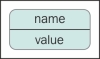
Representing a cell
A counter column is a special purpose cell to keep count. A client application can increment or decrement it by an integer value. Counter columns cannot be mixed with regular or any other cell types (as of Cassandra v2.0.9). So, a counter column always lives in a table that has all the cells of type counter. Let's call this type of table a counter table. When we have to use a counter, we either plug it into an existing counter table or create a separate table with columns (CQL3 columns) as the counter type.
Counters require tight consistency, and this makes it a little complex for Cassandra. Under the hood, Cassandra tracks distributed counters and uses system-generated timestamps. So clock synchronization is crucial.
The counter tables behave a little differently than the regular ones. Cassandra makes a read once in the background when a write for a counter column occurs. So it reads the counter value before updating, which ensures that all the replicas are consistent. Since we know this little secret, we can leverage this property while writing since the data is always consistent. While writing to a counter column, we can use a consistency level of ONE. We know from Chapter 2, Cassandra Architecture, in the Replication topic that the lower the consistency level, the faster the read/write operation. The counter writes can be very fast without risking a false read.
Note
Clock synchronization can easily be achieved with NTPD (http://www.ntp.org). In general, it's a good idea to keep your servers in sync.
Here's an example of a table with counter columns in it and the way to update it:
cqlsh:mastering_cassandra> CREATE TABLE demo_counter_cols (city_name varchar PRIMARY KEY, count_users counter, count_page_views counter);

cqlsh:mastering_cassandra> UPDATE demo_counter_cols SET count_users = count_users + 1, count_page_views = count_page_views + 42 WHERE city_name = 'newyork';

cqlsh:mastering_cassandra> UPDATE demo_counter_cols SET count_users = count_users + 13  WHERE city_name = 'washingtondc';

cqlsh:mastering_cassandra> UPDATE demo_counter_cols SET count_users = count_users + 1, count_page_views = count_page_views + 0 WHERE city_name = 'baltimore';

cqlsh:mastering_cassandra> SELECT * FROM demo_counter_cols;

 city_name    | count_page_views | count_users
--------------+------------------+-------------
 washingtondc |             null |          13
    baltimore |                0 |           1
      newyork |               42 |           1

(3 rows)

cqlsh:mastering_cassandra> UPDATE demo_counter_cols SET count_page_views = count_page_views - 22 WHERE city_name = 'newyork';

cqlsh:mastering_cassandra> SELECT * FROM demo_counter_cols;
 city_name    | count_page_views | count_users
--------------+------------------+-------------
 washingtondc |             null |          13
    baltimore |                0 |           1
      newyork |               20 |           1

(3 rows)
A couple of things to notice here. First, instead of using the INSERT statement, we have used the UPDATE statement to insert the data. If you try to insert, it will fail with an error saying, Bad Request: INSERT statement are not allowed on counter tables, use UPDATE instead. Second, an uninitiated column is set to null by default. You can initiate to any value just by passing an appropriate value in the UPDATE statement.
Note
Note that counter updates are not idempotent. In the event of a write failure, the client will have no idea if the write operation succeeded. A retry to update the counter columns may cause the columns to be updated twice—leading to the column value to be incremented or decremented by twice the value intended.
Every once in a while, you find yourself in a situation where the data gets stale after a given time, and you want to delete it because it does not have a future value or will possibly mess up with the result set. One such example could be a user session object or a password reset request that expires in a day, or maybe you are streaming out word frequency analysis on tweets posted in the last week (moving average). Cassandra gives you the power to make any cell (and hence row) expire after a given time. And if later, before the data is expired, you want to further change the expiry time, you can do that too. This expiry time is commonly referred to as TTL.
On insertion or the update of a TTL-containing cell, the coordinator node sets a deletion timestamp by adding the current local time to the TTL provided. The column expires when the local time of a querying node goes past the set expiration timestamp. The deleted node is marked for deletion with a tombstone and is removed during a compaction after the expiration timestamp or during repair. Expiring columns take 8 bytes of extra space to record the TTL. Here's an example:
# Create a regular table
cqlsh:mastering_cassandra> CREATE TABLE demo_ttl ( id int PRIMARY KEY, expirable_col varchar, column2 int );

# Insert data as usual
cqlsh:mastering_cassandra> INSERT INTO demo_ttl (id, expirable_col, column2) VALUES (1, 'persistent_row', 10);

# Insert a row with TTL equals to 30 seconds
cqlsh:mastering_cassandra> INSERT INTO demo_ttl (id, expirable_col, column2) VALUES (2, 'row_with_30sec_TTL', 30) using TTL 30;
# Observe decreasing TTL with time
cqlsh:mastering_cassandra> SELECT ttl(expirable_col), ttl(column2) FROM demo_ttl WHERE id = 2;

 ttl(expirable_col) | ttl(column2)
  --------------------+--------------
                 23 |           23

  (1 rows)

cqlsh:mastering_cassandra> SELECT ttl(expirable_col), ttl(column2) FROM demo_ttl WHERE id = 2;

 ttl(expirable_col) | ttl(column2)
--------------------+--------------
                  2 |            2

(1 rows)

# The row is deleted
cqlsh:mastering_cassandra> SELECT ttl(expirable_col), ttl(column2) FROM demo_ttl WHERE id = 2;

(0 rows)

# No row, no TTL, obviously
cqlsh:mastering_cassandra> SELECT ttl(expirable_col), ttl(column2) FROM demo_ttl;

 ttl(expirable_col) | ttl(column2)
--------------------+--------------
               null |         null

(1 rows)

# The TTL is not carried forward to new values on the same row that had a TTL previously
cqlsh:mastering_cassandra> INSERT INTO demo_ttl (id, expirable_col, column2) VALUES (2, 'single_cell_TTL', 30);

cqlsh:mastering_cassandra> SELECT ttl(expirable_col), ttl(column2) FROM demo_ttl WHERE id = 2;

 ttl(expirable_col) | ttl(column2)
--------------------+--------------
               null |         null

(1 rows)

# Setting TTL is CELL LEVEL, so you need to set it individually
cqlsh:mastering_cassandra> UPDATE demo_ttl USING TTL 60 SET expirable_col = 'single_cell_TTL' WHERE id = 2;

cqlsh:mastering_cassandra> SELECT ttl(expirable_col), ttl(column2) FROM demo_ttl WHERE id = 2;

 ttl(expirable_col) | ttl(column2)
--------------------+--------------
                 56 |         null

(1 rows)

# Only the cell with TTL is deleted
cqlsh:mastering_cassandra> SELECT * FROM demo_ttl;

 id | column2 | expirable_col
----+---------+----------------
  1 |      10 | persistent_row
  2 |      30 |           null

(2 rows)

# You CANNOT really just update TTL of a whole row without actually manually updating each cell!
cqlsh:mastering_cassandra> UPDATE demo_ttl USING TTL 60 WHERE id = 2;

Bad Request: line 1:29 mismatched input 'WHERE' expecting K_SET

# You can reset a TTL
cqlsh:mastering_cassandra> INSERT INTO demo_ttl (id, expirable_col, column2) VALUES (3, 'some_more_time_please', 40);
cqlsh:mastering_cassandra> UPDATE demo_ttl USING TTL 30 SET expirable_col = 'some_more_time_please' WHERE id = 3;

cqlsh:mastering_cassandra> SELECT ttl(expirable_col) FROM demo_ttl WHERE id = 3;

 ttl(expirable_col)
--------------------
                 12

(1 rows)

# Do the same things that you do to assign a TTL
cqlsh:mastering_cassandra> UPDATE demo_ttl USING TTL 60 SET expirable_col = 'some_more_time_please' WHERE id = 3;

cqlsh:mastering_cassandra> SELECT ttl(expirable_col) FROM demo_ttl WHERE id = 3;

 ttl(expirable_col)
--------------------
                 59

(1 rows)

#Dismiss a TTL by setting it to zero
cqlsh:mastering_cassandra> UPDATE demo_ttl USING TTL 60 SET expirable_col = 'some_more_time_please' WHERE id = 3;

cqlsh:mastering_cassandra> SELECT ttl(expirable_col) FROM demo_ttl WHERE id = 3;

 ttl(expirable_col)
--------------------
                 55

(1 rows)

cqlsh:mastering_cassandra> UPDATE demo_ttl USING TTL 0 SET expirable_col = 'some_more_time_please' WHERE id = 3;

cqlsh:mastering_cassandra> SELECT ttl(expirable_col) FROM demo_ttl WHERE id = 3;

 ttl(expirable_col)
--------------------
               null

(1 rows)
The following are a few things to be noted about expiring columns:
- The TTL is in seconds, so the smallest TTL can be 1 second
- You can change the TTL by updating the column (that is, read the column, update the TTL, and insert the column)
- You can dismiss TTL by setting it to zero
- Although the client does not see the expired column, the space is kept occupied until the compaction process after
gc_grace_secondsis triggered; but note that tombstones take a rather small space
Expiring cells can have some good uses; they remove the need for constantly watching cron-like tasks that delete the data that has expired or is not required any more. For example, an expiring shopping coupon or a user session can be stored with a TTL.
Note
Where is my super column?
People who have used Cassandra in version 1.1 or older must have heard of a super column which is nothing but a cell that can have subcells. It was overly hyped and was considered bad practice, the reason being, it was not automatically sorted like other cells. You have to fetch all the subcolumns and it was adding unnecessary special casing in the Cassandra code base. From Cassandra 1.2 onward, super columns were removed. The Thrift request was still supported in 1.2, but it was internally using collections instead of subcolumns.
As we will see, Cassandra 2.0 and later versions have much richer, better, and faster ways to do all that you could do with super columns and more.
In CQL3 grammar, the column family and table are used interchangeably. In this particular section, when we say column family we mean the older representation of data storage. This representation is much closer to how the data is stored in Cassandra. We will discuss how this representation maps to the new CQL3 representation when we learn about CQL3 later in this chapter. Understanding this section will help you to understand concepts such as wide rows, and how collections work in CQL3.
A column family is a collection of rows where each row is a key-value pair. The key to a row is called a row key and the value is a sorted collection of cells. Essentially, a column family is a map with its keys as row keys and values as an ordered collection of cells.
Internally, each column family is stored in a file of its own, and there is no relational integrity between two column families. So you should keep all related information that the application might require in the column family.
In a column family, the row key is unique and serves as the primary key. It is used to identify and get/set records to a particular row of a column family.
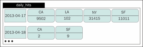
Although a column family looks like a table from the relational database world, it is not. When you use CQL, it is treated as a table, but having an idea about the underlying structure helps in designing—how the cells are sorted, sliced, and persisted, and the fact that it's a schema-free map of maps. A dynamic column family showing daily hits on a website is displayed in the following figure. Each column represents a city and the column value is the number of hits from that city:
You can define a column family in such a way that it behaves as a standard RDBMS table or as a sequence of key-value pairs. The former is called static or narrow column family and the latter is known as dynamic or wide row column family. The concept of dynamic column family (table) is not overly stated in CQL3, but whenever you create a table with a compound key, you get a wide row. Let's demonstrate that.
To show how static tables and wide row tables differ in their underlying presentations, we will use cassandra-cli, a previous generation utility that uses the Thrift protocol to connect to Cassandra and assumes the column families are just sorted hash maps containing sorted hash maps.
Here's how you create a static column family:
# Using cqlsh
cqlsh:mastering_cassandra> CREATE TABLE demo_static_cf (id int PRIMARY KEY, name varchar, age int);

cqlsh:mastering_cassandra> INSERT INTO demo_static_cf (id, name, age) VALUES ( 1, 'Jennie', 39);

cqlsh:mastering_cassandra> INSERT INTO demo_static_cf (id, name, age) VALUES ( 2, 'Samantha', 23);

cqlsh:mastering_cassandra> SELECT * FROM demo_static_cf;

 id | age | name
----+-----+----------
  1 |  39 |   Jennie
  2 |  23 | Samantha

(2 rows)# View using cassandra-cli
[default@mastering_cassandra] LIST demo_static_cf;
Using default limit of 100
Using default cell limit of 100
-------------------
RowKey: 1
=> (name=, value=, timestamp=1410338723286000)
=> (name=age, value=00000027, timestamp=1410338723286000)
=> (name=name, value=4a656e6e6965, timestamp=1410338723286000)
-------------------
RowKey: 2
=> (name=, value=, timestamp=1410338757669000)
=> (name=age, value=00000017, timestamp=1410338757669000)
=> (name=name, value=53616d616e746861, timestamp=1410338757669000)
2 Rows Returned.
Elapsed time: 197 msec(s).Pretty neat! Two rows with two different unique keys go into two different rows. So, the CQL representation is the same as the way the data is actually stored (Thrift representation). But this would not hold true for tables with a compound key. Here's how you create a table with a compound key:
# Using cqlsh
cqlsh:mastering_cassandra> CREATE TABLE demo_wide_row (id timestamp , city varchar, hits counter, primary key(id, city)) WITH COMPACT STORAGE;

cqlsh:mastering_cassandra> UPDATE  demo_wide_row SET hits = hits + 1 WHERE id = '2014-09-04+0000' AND city = 'NY';

cqlsh:mastering_cassandra> UPDATE  demo_wide_row SET hits = hits + 5 WHERE id = '2014-09-04+0000' AND city = 'Bethesda';

cqlsh:mastering_cassandra> UPDATE  demo_wide_row SET hits = hits + 2 WHERE id = '2014-09-04+0000' AND city = 'SF';

cqlsh:mastering_cassandra> UPDATE  demo_wide_row SET hits = hits + 3 WHERE id = '2014-09-05+0000' AND city = 'NY';

cqlsh:mastering_cassandra> UPDATE  demo_wide_row SET hits = hits + 1 WHERE id = '2014-09-05+0000' AND city = 'Baltimore';

cqlsh:mastering_cassandra> SELECT * FROM demo_wide_row;

 id                       | city      | hits
--------------------------+-----------+------
 2014-09-05 05:30:00+0530 | Baltimore |    1
 2014-09-05 05:30:00+0530 |        NY |    3
 2014-09-04 05:30:00+0530 |  Bethesda |    5
 2014-09-04 05:30:00+0530 |        NY |    1
 2014-09-04 05:30:00+0530 |        SF |    2

(5 rows)
One would expect that there should be five rows on a disk, but there are actually just two rows one for each unique ID. Here is what you get from cassandra-cli:
[default@mastering_cassandra] LIST demo_wide_row;

Using default limit of 100
Using default cell limit of 100
-------------------
RowKey: 2014-09-05 05:30+0530
=> (counter=Baltimore, value=1)
=> (counter=NY, value=3)
-------------------
RowKey: 2014-09-04 05:30+0530
=> (counter=Bethesda, value=5)
=> (counter=NY, value=1)
=> (counter=SF, value=2)

2 Rows Returned.

Elapsed time: 194 msec(s).
So why this discrepancy? We know that the data model of Cassandra is basically a hash map. When you create a table with a compound key, the first component of the key is treated as a row key and other components are treated as the cell name. This provides a couple of major benefits because unlike the row key, which is distributed across the machines, rows stay on one machine and are sorted by names. So, you can perform range queries as follows:
cqlsh:mastering_cassandra> SELECT * FROM demo_wide_row WHERE id = '2014-09-04+0000' AND city > 'Baltimore' AND city < 'Rockville';

 id                       | city     | hits
--------------------------+----------+------
 2014-09-04 05:30:00+0530 | Bethesda |    5
 2014-09-04 05:30:00+0530 |       NY |    1

(2 rows)
However, this is not the only way to get range queries working. We will say later that we could do the same using a secondary index. So, why wide rows? Wide rows are traditionally useful for things like data series. An example of data series is time series where data is ordered by time such as a Twitter feed or Facebook timeline. In these cases, you may have user_id as a row key (partition key, which is the first component of a composite key), and timestamp as the cell names (the second component of a composite key), and the cell value is the data (a tweet or a timeline item).. It can be used to store sensor data in your Internet of Things application where row-key, cell name, and cell data are sensor ID, timestamp of data generated, and data from the sensor, respectively.
Keyspaces are the outermost shells of Cassandra containers. It is the logical container of tables. It can be roughly imagined as a database of a relational database system. Its purpose is to group tables. In general, one application uses one keyspace, much like RDBMS.
Keyspaces hold properties such as replication factors and replica placement strategies, which are globally applied to all the tables in the keyspace. Keyspaces are global management points for an application.
Cassandra supports all data types any standard relational database supports and more. Here's the list of data types Cassandra 2.x supports:
Apart from these data types, you can mix and match these data types to create your own data type much like a struct in the C language. We will see this later in this chapter when we discuss CQL3.
A primary key or row key is the unique identifier of a row, in much the same way as the primary key of a table from a relational database system. It provides quick and random access to the rows. Since the rows are sharded (distributed) among the nodes, and each node just has a subset of rows, the primary keys are distributed too. Cassandra uses the partitioner (cluster-level setting) and replica placement strategy (keyspace-level setting) to locate the nodes that own a particular row. On a node, an index file and sample index is maintained locally and can be looked up via binary search followed by a short sequential read. (For more information, refer to Chapter 2, Cassandra Architecture.)
The problem with primary keys is that their location is governed by partitioners. Partitioners use a hash function to convert a row key into a unique number (called token) and then read/write happens from the node that owns this token. This means that if you use a partitioner that does not use a hash that follows the key's natural ordering, chances are that you can't sequentially read the keys just by accessing the next token on the node.
The following code snippet shows an example of this. The row keys 1234 and 1235 should naturally fall next to each other if they are not altered (or if an order preserving partitioner is used). However, if we take a consistent MD5 hash of these values, we can see that the two values are far away from each other. There's a good chance that they might not even live on the same machine. Here is an example of how two seemingly consecutive row keys have MD5 hash that is far apart:
ROW KEY | MD5 HASH VALUE
--------+----------------------------------
1234    | 81dc9bdb52d04dc20036dbd8313ed055
1235    | 9996535e07258a7bbfd8b132435c5962
Let's take an example of two partitioners: ByteOrderPartitioner that preserves lexical ordering by bytes, and RandomPartitioner that uses an MD5 hash to generate a row key. Let's assume that we have a users_visits table with a row key, <city>_<userId>. ByteOrderPartioner will let you iterate through rows to get more users from the same city in much the same way as a SortedMap interface does (for more detail, visit http://docs.oracle.com/javase/6/docs/api/java/util/SortedMap.html). However, in RandomPartioner, the key being the MD5 hash value of <city>_<userId>, the two consecutive userIds from the same city may be such that there are records for a different city in between. So, we cannot just iterate and expect grouping to work, like accessing entries of HashMap. (Ideally, you would not want to use a row key <city>_<userId> for grouping. You would create a compound key with <city> and <userId>. The purpose of the preceding example was just to show that consecutive row keys may have records between them.)
We will see partitioners in further detail in Chapter 4, Deploying a Cluster. But using the obviously better looking partitioner ByteOrderPartitioner is assumed to be a bad practice. There are a couple of reasons for this; the major reason being an uneven row key distribution across nodes. This can potentially cause a hotspot in the ring.
CQL3 provides a SQL-like grammar to access data in a tabular manner. In the previous section, we saw how the data is actually stored in Cassandra. The CQL representation may not look like that especially when you use a composite key. In this section, we will discuss all the features of CQL3.
In this section, a typographic convention is used to indicate syntactic information. Here's the list of stylization used:
- Capital letter means literal or keyword.
- Curly brackets with the pipe character within them means that you must use at least one of those keywords in the query. Curly brackets are also used to specify a map, but they do not have the pipe character in them and they follow JSON notation.
- Square brackets show options settings.
- Lowercase means variables are to be provided by the developer.
Let's try to interpret an example:
CREATE { KEYSPACE | SCHEMA } [IF NOT EXISTS] keyspace_name

WITH REPLICATION = json_object

[AND DURABLE_WRITES = { true | false }]
The preceding query pattern suggests that after CREATE, we must use either KEYSPACE or SCHEMA followed by an optional IF NOT EXISTS setting, followed by the name of your choosing for the keyspace, followed by WITH REPLICATION. After this, you fill in a JSON object that specifies replication behavior and finally, we may choose to set DURABLE_WRITES. If we do choose to set DURABLE_WRITES, we must assign it a true or a false value.
Keyspace is the logical container of tables just like a databaseor a schema in a RDBMS. Keyspace also holds some of the global settings applied to all the tables in it.
Cassandra needs two things from you to specify when creating a keyspace; one, the name of the keyspace, and the other is the replication strategy. Optionally, you can specify IF EXISTS clause if you are writing a script that adds tables to an existing keyspace and do not want to error out on the first line that creates the keyspace. You may want to specify whether you wanted a durable write. Note that switching off the durable write may be a bad idea. And generally, you would not want to disable durable write. While I agree that there is some performance gain by disabling durable write as it bypasses the commit log, it does so at the cost of possible data loss. You may get some performance gain just by moving commit log to a separate disk by changing the setting in cassandra.yaml. Here is how you create a keyspace:
CREATE { KEYSPACE | SCHEMA } [IF NOT EXISTS]The REPLICATION setting takes a map. If you are using cqlsh, you need to type a JSON object to specify it. This setting is to specify how you want your data to be replicated across the nodes. There are two options to do this: SimpleStrategy and NetworkTopologyStrategy.
SimpleStrategy is used when you have single data center or you want all nodes to be treated as they are in a single data center. In this setting, data is placed on one node and its replica is placed on the consecutive next node when moving clockwise (increasing token number side). SimpleStrategy is specified as follows:
{ 'class' : 'SimpleStrategy', 'replication_factor' : <positive_integer> }Here, <positive_integer> is the number of copies of data you want and it should be greater than zero.
NetworkTopologyStrategy, as the name suggests, stores data depending on how the nodes are placed. Replicas should be stored on nodes that are on different racks in the data center to avoid a failure in case a rack dies. In this strategy, you can specify how many replicas you want in a data center if you have your nodes spanning across various data centers. It may be worth noting that each data center has a full set of data with specified replica. So, if you choose a DC1 to have the replication factor of 2 and DC2 to have the replication factor of 3, the whole corpus exists in DC1 and DC2 with DC1 having two copies of your data and DC2 having three. In the event of a complete data center failure, you can still work from the other data center.
This strategy is a recommended setting for production setup even if you have just one data center to start with. To specify this strategy, you should do the following:
{ 'class' : 'NetworkTopologyStrategy'[, '<datacenter_name>' : <positive_integer>, '<datacenter_name>' : <positive_integer>, ...] }Here are a couple of examples:
# Single data center, replication factor: 3
{ 'class' : 'NetworkTopologyStrategy', 'DC1' : 3}

# Three data centers, with RF as 3, 2, and 1
{ 'class' : 'NetworkTopologyStrategy', 'DC_NY' : 3, 'TokyoDC' : 2, 'DC_Hadoop': 1}

# Two data centers with three replica each
{ 'class' : 'NetworkTopologyStrategy', 'DC1' : 3, 'DC2' : 3}
Now, how would each node know which data center it belongs to? Snitch; you configure snitch in Cassandra's configuration file cassandra.yaml. We have already seen snitch and how it works and configured in Chapter 2, Cassandra Architecture, and we will see them again in Chapter 4, Deploying a Cluster.
Note that while you may still create a keyspace without any data center configuration when using NetworkTopologyStrategy, you may get an error when writing data to Cassandra.
Here are two examples of what your standard keyspace creation looks like:
# Keyspace with SimpleStrategy
CREATE KEYSPACE IF NOT EXISTS demo_keyspace
WITH REPLICATION = { 'class' : 'SimpleStrategy', 'replication_factor' : 3 }

# Keyspace with NetworkTopologyStrategy
CREATE KEYSPACE IF NOT EXISTS demo_keyspace1
WITH REPLICATION = {'class': 'NetworkTopologyStrategy', 'DC1': 3, 'DC2': 1}

# Keyspace with no durable writes
CREATE KEYSPACE IF NOT EXISTS demo_keyspace2
WITH REPLICATION = {'class': 'NetworkTopologyStrategy', 'DC1': 3, 'DC2': 1}
AND DURABLE_WRITES = 'false'
Note that class and replication_factor in the REPLICATION setting must be in lowercase.
You can alter keyspace properties like REPLICATION and DURABLE_WRITES, but the names cannot be altered. Here is the CQL syntax for that:
ALTER {KEYSPACE | SCHEMA} keyspace_name
WITH {
  REPLICATION = json_object |
  DURABLE_WRITES =  {true | false} |
  REPLICATION = json_object AND DURABLE_WRITES = {true | false}
}Table creation in CQL3 is similar to how it's done in SQL. At the very least, you need to specify the table name, the name and types of the columns, and the primary key. The primary key can be single valued (made of a single column) or composite (made of more than one column). For more detail on keys, refer to the A brief introduction to the data model section in Chapter 1, Quick Start. In the former case, the primary key works as a partition key (or shard key). So, rows of such a table are distributed across the nodes based on the hash value of the primary key. In the latter case, where primary key constitutes of more than one column, the first column works as partition key. That means rows with same partition key stay in one wide row. (Refer to the The column family section.) This can be handy when you want to group things naturally. The following code snippet can be used to create a table:
CREATE TABLE [ IF NOT EXISTS ] [keyspace_name.]table_name
( column_definition, column_definition, ...)
[WITH property [ AND property ... ]]
Column definition, in most of the common cases, will be as follows:
column_name column_type [STATIC | PRIMARY KEY]
Let's take a look at the following example:
CREATE TABLE mytab (id int PRIMARY KEY, name varchar, article text, is_paying_user boolean, phone_numbers set <varchar>);
You may define PRIMARY KEY separately, like we do in the case of the compound key:
CREATE TABLE team_match (city varchar, team_name varchar, is_participating boolean, player_id set <int>, PRIMARY KEY(city, team_name));
With Cassandra 2.1, you could create tables that have custom types, and on the same working principle it lets you create tuples. There is a special way to declare a tuple or custom type. You use the frozen keyword for them. The pattern is as follows:
column_name frozen<tuple<type [, type, ...]>> [PRIMARY KEY]
column_name frozen<user_defined_type> [PRIMARY KEY]
So, what does frozen signify? Cassandra serializes the tuple or user defined type into one cell. It may be noted that although the collections live in separate cells, if you have nested collections, the inner collections are serialized into one cell. This means when you update a user defined type or tuple, it pulls the whole thing, updates it, and inserts it again. But Cassandra might allow individual updates in version 3.0 and above. So, the frozen keyword is just a safety feature to avoid conflicts when you migrate to the third version. For now, you cannot create a column of user defined type, or tuple type without adding the frozen keyword. For more details on frozen, look at the Jira ticket (https://issues.apache.org/jira/browse/CASSANDRA-7857). Let's see the frozen keyword in action:
cqlsh:demo_cql> CREATE TYPE address (line1 varchar, line2 varchar, city varchar, state varchar, postalcode int);

cqlsh:demo_cql> CREATE TABLE customer (id int PRIMARY KEY, name varchar, addr address);

code=2200 [Invalid query] message="Non-frozen User-Defined types are not supported, please use frozen<>"

cqlsh:demo_cql> CREATE TABLE customer (id int PRIMARY KEY, name varchar, addr frozen<address>);

cqlsh:demo_cql> CREATE TABLE purchase_ability(id int PRIMARY KEY, customer_id int, purchase_rating tuple<float, float, int, boolean>);

code=2200 [Invalid query] message="Non-frozen tuples are not supported, please use frozen<>"

cqlsh:demo_cql> CREATE TABLE purchase_ability(id int PRIMARY KEY, customer_id int, purchase_rating frozen<tuple<float, float, int, boolean>>);
You can specify a non-clustering column as static and this column stays static across all the rows with the same partition key (row key). This only applies to the columns not involved in compound key. The static column does not make sense in a setting where you do not have a compound key because in those cases, you have row key as the primary key and hence each row lives in a separate partition, so each column is essentially a static column. Here's an example:
# We wanted to have one university per ID
CREATE TABLE static_col (id int, city varchar, university varchar static, name varchar, PRIMARY KEY(id, city));

# Insert some data
INSERT INTO static_col (id, city, university, name ) VALUES ( 1, 'Seattle', 'Seattle University', 'Barry Kriple'),
INSERT INTO static_col (id, city, university, name ) VALUES ( 2, 'Washington', 'Washington University', 'Rose Byrne'),

INSERT INTO static_col (id, city, university, name ) VALUES ( 1, 'Washington', 'Seattle University', 'Nick Jonas'),

# So far so good
SELECT * FROM static_col;


 id | city       | university            | name

----+------------+-----------------------+--------------
  1 |    Seattle |    Seattle University | Barry Kriple
  1 | Washington |    Seattle University |   Nick Jonas
  2 | Washington | Washington University |   Rose Byrne

(3 rows)

# Just insert another record to id=1 with a different university name
INSERT INTO static_col (id, city, university, name ) VALUES ( 1, 'New York', 'Coursera', 'John Hacker Doe'),

# All the records in that row key are updated
cqlsh:demo_cql> SELECT * FROM static_col;


 id | city       | university            | name

----+------------+-----------------------+-----------------
  1 |   New York |              Coursera | John Hacker Doe
  1 |    Seattle |              Coursera |    Barry Kriple
  1 | Washington |              Coursera |      Nick Jonas
  2 | Washington | Washington University |      Rose Byrne

(4 rows)
The static column can be useful when you want to store a common global record of a column across all the records that share the same row key. It can be thought of as a static variable in Java, which is shared among all the instances of the class. An application of such a case could be a game where you are given initial credit coins, and you can use these coins to purchase things in the game. When you buy something, a purchase record is added with balance_coins as the static column. However, one might argue to use counter, which makes sense. Another example could be a static Set<text> to keep a set of ever changing tags of a product of a category available to all the products. For more rationale on static type, you can review the Jira ticket for this feature at https://issues.apache.org/jira/browse/CASSANDRA-6561.
Table or column family is the center of the Cassandra universe. CQL3 provides you with options to tweak things to meet your requirements—both performance and functional, both. Here's a list of attributes that you set as your table properties.
As discussed in Chapter 2, Cassandra Architecture, the bloom filter is an in memory data structure to test whether the requested row exists in an SSTable before making a disk seek. It's a neat idea to avoid hitting disk read and hence reduces latency. The bloom filter is a probabilistic data structure and it may return a false positive result when asked. That means, when you ask a bloom filter if the SSTable it is associated with has a row it may say yes, while the SSTable does not have the row. But if it says no, the SSTable definitely does not have the row. You can configure the probability of getting the false positive result by setting bloom_filter_fp_chance. The tradeoff is that the lower the value of false-positive probability, the higher the amount of memory the bloom filter will consume. So, you can set bloom_filter_fp_chance to 0 for no false positive result, which will result in the largest bloom filter array for the table.
On the other hand, you can set it to 1, to say you want all false positive results, basically disabling the bloom filter. In practice, you would not want any of those extreme cases. The recommended and default value is 0.01 (if you choose LeveledCompactionStrategy, the default value get set to 0.1). Ideally, you wouldn't touch this configuration unless you are really concerned about 10 percent reads that might be hitting the disk. Let's take a look at the following example:
CREATE TABLE tiny_tiny_table (
  tab_id uuid,
  tab_details text,
  PRIMARY KEY (tab_id)
) WITH bloom_filter_fp_chance = 0.001;
If you have caching enabled in cassandra.yaml, Cassandra automatically caches data based on frequency of its access and size of the data. You can tune it for individual tables if you want. All you need to do is to specify caching in table creation or update CQL.
There are two types of caching: row caching, which is similar to the caching that object-relational mappers provide on top of RDBMS. Row caching caches the whole row and returns it from the memory if it is cached. The data gets cached after its first access. The other type of caching is key caching where just the key is cached in the memory. It takes much smaller memory, so we can have lots of keys caches without burning a lot of memory. Unlike row caching, this does require a disk seek to read the actual data. But data retrieval is much more efficient with key caching enabled than without it. It is suggested to keep key caching on unless you have a specific reason not to.
If you are using Cassandra 2.1, you can set both the caching individually using the following property:
caching = { 'keys' : '{NONE|ALL}', 'rows_per_partition' : '{NONE|ALL|positive_int}' };Here's an example:
CREATE TABLE searched_pages (
  page_id uuid,
  page_text text,
  metadata text,
  advertisement_count int,
  PRIMARY KEY (page_id)
) WITH caching = { 'keys' : 'ALL', 'rows_per_partition' : '31415' };
For Cassandra 2.0.x releases, the query looks a bit different. You specify it as caching = {'all'|'keys_only'|'rows_only'|'none'}.
Here's an example:
CREATE TABLE searched_pages (
  page_id uuid,
  page_text text,
  metadata text,
  advertisement_count int,
  PRIMARY KEY (page_id)
) WITH caching = 'keys_only';
As you can see here, in Cassandra 2.0.x, we cannot set the number of rows per partition to be cached. By default, Cassandra has key caching enabled.
You can add comments to describe the specifics of a table to clarify the purpose of the table. Here's an example:
CREATE TABLE pigeon_hole (
  pigeon_id uuid,
  pigeon_offense text,
  pigeon_age int,
  is_it_a_fun_pigeon boolean,
  PRIMARY KEY(pigeon_id)
) WITH comment = 'Pigeon hole is a table for criminal pigeons. They cannot see or talk to each other but if they are fun, we may want to feed them once in a while';
As we know from Chapter 2, Cassandra Architecture, Memtables eventually get flushed to disk as immutable SSTables. But with time, we get lots of SSTables that may make data retrieval slow, and data mutation operations such as update and delete render rows living in an old SSTable useless. Cassandra performs compaction where it merges SSTables to solve these issues. We will see compaction in a little more detail in Chapter 5, Performance Tuning. For now, you should know that there are two types of compaction strategies:
An example of setting a compaction strategy is as follows:
CREATE TABLE compaction_demo (id uuid PRIMARY KEY, name varchar)
WITH
COMPACTION  = {
'class': 'SizeTieredCompactionStrategy',
'tombstone_compaction_interval':43200,
'tombstone_threshold': 0.1
};
As you can see in the preceding code snippet, we have specified some other properties that are related to compaction in the query. Cassandra provides a very detailed configuration parameter to tweak the way you want the compaction process to take place. Here's the list of properties that you can specify within the JSON object for the COMPACTION keyword:
enabled: This takes a Boolean value. This property tells Cassandra to enable or disable compaction on the particular table. You would probably never want to disable it, so likely you are not going to use it.tombstone_threshold: This is the ratio of cells (columns) in an SSTable that are eligible for deletion (garbage collectable) to the total number of columns in the SSTable. Essentially, it is the percentage of discarded columns in the SSTable expressed in decimal. By default, when 20 percent of SSTable columns become garbage collectable, it becomes a candidate fortombstone_compaction.tombstone_compaction_interval: This is the minimum amount of wait time (in seconds) before the SSTable is considered for tombstone compaction. Iftombstone_thresholdis reached, the SSTable is compacted; otherwise, Cassandra retries again aftertombstone_compaction_interval. So, it may not be wise to set this value too small. The default is 86400 seconds (one day).unchecked_tombstone_compaction: If the data from the partition that the tombstone belongs to exists in other data files, the tombstone cannot be discarded; it works as an indicator of deletion. This check is performed every time before a tombstone compaction is attempted. This is extra work and is exactly why you would not want to keeptombstone_compaction_intervaltoo low. By setting this option astrue, you are telling Cassandra to try to compact without performing this check. Compaction may fail in this case, but if you have a situation where you have immutable rows that get discarded as a whole, you may opt for this option.min_sstable_size(specific toSizeTieredCompactionStrategy): This defines SSTables of similar sizes into one big SSTable. So, one can think of the compaction process as bucketed or batch process where SSTables that fall into one bucket get merged into one. If your SSTables are really small, you may end up in many tiny buckets, which may be inefficient.min_sstable_sizeis to specify the minimum size of SSTable, below which, all the SSTables are assumed to be in one bucket and compacted. The unit ofmin_sstable_sizeis bytes and the default value is 50 MB.min_thresholdandmax_threshold(specific toSizeTieredCompactionStrategy): This defines the minimum number of similar sized SSTables to start compaction.max_thresholdis the maximum number of SSTables to consider in a compaction process. The default value ofmin_thresholdis 4 and the default value ofmax_thresholdis 32.bucket_highandbucket_low(specific toSizeTieredCompactionStrategy): When we mentioned similar sizes in the previous point, what we meant is explained here. A set of SSTables are assumed to be in the same bucket to be compacted if their size lies within the range described by this formula:[average_size*bucket_low, average_size*bucket_high]. Ideally,bucket_lowshould be a positive decimal fraction value less than one, andbucket_highis a decimal fraction more than one. Default values forbucket_lowandbucket_highare 0.5 and 1.5 respectively.cold_reads_to_omit(specific toSizeTieredCompactionStrategy): Cassandra keeps track of which SSTable contributes to how many reads. So there may be cases where some SSTables contribute very little to nothing to the reads. It may not be worth the additional effort to compact those "cold" SSTables because they are accessed once in a while. For example, you have a table that has total 200 reads per second overall, of which 100 are contributed by SSTable S1, 85 by S2, 10 by S3, and 5 by S4. If you havecold_reads_to_omitas 0.1, then SSTables that cumulatively contribute to 200*0.1 or 20 reads will not be considered for compaction. Adding from the tiniest ones, S4 and S3 contribute to only 15 reads per second, so they will not be considered a candidate for compaction. Values forcold_reads_to_omitcan be anything between 0.0 and to 1. However, you would not want to set it to 1, ignoring all the SSTables. Setting it to zero disabled discriminating the SSTables' eligibility to compact based on its contribution in reads. The default in Cassandra 2.1 and onwards is 0.05 and in the previous versions it is 0.sstable_size_in_mb(specific toLeveledCompactionStrategy): This is the target size for SSTable inLeveledCompactionStrategy. Cassandra tries to keep SSTable size less than or equal to this value, but SSTable may be larger than this value in exceptional cases where a partition key holds very large data. The default value is 160 MB.Compression: There are three compression algorithms available in Cassandra out of the box,LZ4Compressor,SnappyCompressor, andDeflateCompressor, in the decreasing order of read performance and increasing order disk space saving. So, why would one want a degraded performance for disk space? Consider a case where you have a table just for archival purposes. Here's an example of setting compression:CREATE TABLE compression_demo (id uuid PRIMARY KEY, name varchar) WITH COMPRESSION = { 'sstable_compression': 'SnappyCompressor', 'chunk_length_kb': 128 };
To disable compression, use the empty string ('') as the value for the sstable_compression attribute. Compression has a couple of other properties that can be tuned:
chunk_length_kb: A chunk is the minimum quantum of data that is read by Cassandra. Depending on how much data is read on an average and the mean size of the rows of the table, this property may be tweaked. The higher value for this may improve compression performance, but it will also increase the minimum size of data read. In general, you wouldn't touch the default value of 64, unless you are familiar with data and its access pattern in the future.crc_check_chance: Cyclic Redundancy Check or CRC is a way to validate if the uncompressed data is exactly the same as the original. In cases when you have compression enabled for a table, each compressed block holds a checksum for CRC to avoid any data corruption. This property tells the probability by which reads are verified for any errors. By default, it is set to 1, so all reads are first validated for data integrity. If it is set to 0.25, every fourth read is validated.time_to_live: You have seen previously in this chapter that you can set TTL for individual row or cell, but there may be cases where you want all the rows to be deleted after some time. For example, if you have a table that is used to aggregate data for the last 24 hours, you may just want to keep the data for the last 24 hours or may be a little bit longer. You can do this by specifyingdefault_time_to_livein seconds when creating or updating a table. To disable TTL, set this property to 0. The default is zero.CREATE TABLE ttl_demo (id uuid PRIMARY KEY, name varchar) WITH default_time_to_live = 86400;
read_repair_chance: Thedc_local_read_repair_chancespecifies the probability of performing a repair (making all replicas consistent) only in the data center that received the read request. If it is set to 0.25, every fourth read request will sync the whole data center. The default is 0.1.There is a global version of
dc_local_read_repair_chance, that is,read_repair_chance. Theread_repair_chancedenotes the probability by which repairs across all the data centers take place. By default, this value is set to zero.gc_grace_seconds: When a cell or a row is deleted, it is marked so by writing a tombstone. These tombstones aren't immediately removed on compaction. Tombstones live tillgc_grace_secondsbefore they become eligible to be removed. The reason for the wait is to avoid deleted data from respawning. You may ask how does it respawn. Let us assume that tombstones get removed immediately. This is fine when all nodes are up. In a case where there is a dead node carrying the data that was deleted, comes an issue. When the dead node comes back to the life, it communicates with the other nodes to repair data. Since there is no information about the deleted data as there is no tombstone, the dead node thinks it has the only copy of the data, and it updates all the other nodes with the data that should have been deleted. This would cause resurrection of a deleted record, which would be undesired. The defaultgc_grace_secondsis 864,000 or 10 days, which is probably enough time to notice a dead node and take appropriate action before garbage collection begins. On a single node setup this may be set to zero.index_interval: Each SSTable has an index summary loaded in the memory that keeps a sample of row keys index in that SSTable. Cassandra 2.0.x releases have a parameter namedindex_intervalthat basically dictates the number of primary key or row key skipped in the sample. The default value for this is 128. This means that the index of every 128th record in the SSTable is kept in memory. Talking of trade off, obviously the smaller theindex_interval, the larger the number of rows indexes store in memory, which means a larger memory footprint and faster row retrieval.Note
Cassandra 2.1.0 and onwards, introduced two intervals:
min_index_intervalandmax_index_interval. This is slightly smarter than the previous version. Based on the frequency of access of an SSTable, it determines the index interval to use. So, for a rarely accessed SSTable, the index interval will be equal tomax_index_interval, and for an in-demand SSTable, the index interval will bemin_index_interval. For the SSTables that are neither in high demand nor in low demand, the index interval will be set to somewhere between the min and max values. The index interval also depends on the availability of free memory in the index summary memory pool.memtable_flush_period: Memtables are serialized to SSTable after a time period defined by this attribute. This represents the number of milliseconds after which a Memtable is forced to be flushed to the disk. The default is zero.replicate_on_write: This is the only feature in Cassandra 2.0.x. Whenreplicate_on_writeis set totrue, the data is written to all the replicas irrespective of the consistency level setting. It is true for counter tables by default.speculative_retry: Cassandra makes only as many requests as consistency level dictates. If a node dies during a read, Cassandra waits till timeout and then responds with a timeout error message. Withspeculative_retry, Cassandra avoids failure by sensing the unusual delay that a replica takes, and retries on a different replica. Here are the available settings:ALWAYS: Cassandra reads from all the replicas and returns as soon as the consistency level is met.Xpercentile: Retry triggers if the read operation takes more time than what the fastest X percent of reads took in the past. For example, if it is set to99percentile, the retry will trigger if a read operation takes more time than the fastest 99 percent of the queries took.Xms: Retry triggers if the read did not return after X milliseconds of sending the request. So, if you wanted a speculative retry to happen if a replica did not respond in under 42 ms, setspeculative_retryto42 ms.NONE: No retries.
Here's an example:
CREATE TABLE speculative_retries_demo (id uuid PRIMARY KEY, name varchar)
WITH
speculative_retry = '99percentile';
Altering a table is similar to creating one. You can add, rename, change type, drop columns, and you can also change various table properties that we saw in the previous section. Let's take a simple table and play with it:
CREATE TABLE modify_me (id uuid PRIMARY KEY, name varchar);
Adding a column has a syntax as follows:
ALTER TABLE table_name ADD new_column_name column_type;
However, you cannot mix a counter column in a non-counter table. Let's take a look at the following examples:
ALTER TABLE modify_me ADD phone_numbers map <varchar, varchar>;

ALTER TABLE modify_me ADD count_sheep counter;

<ErrorMessage code=2300 [Query invalid because of configuration issue] message="Cannot add a counter column (count_sheep) in a non counter column family">
Renaming has very limited capability. Cassandra 2.1.0 only allows renaming columns that are a part of a primary key. The syntax is as follows:
ALTER TABLE table_name RENAME old_name TO new_name;
Changing the data type of a column is possible as long the new data type is compatible with the old (existing) one, ideally superset. For example, ASCII can be converted to VARCHAR and VARCHAR to TEXT. Here's an example:
# A table with a clustering column and index
CREATE TABLE type_changer (id int, name ascii, age ascii, primary key(id, age));

CREATE INDEX tc_idx ON type_changer (name);


# Alter the clustering column
ALTER TABLE type_changer ALTER age TYPE varchar;


# Insert some data
INSERT INTO type_changer (id, age, name) VALUES ( 1, '12', 'Mercedes'),


# Alter everything
ALTER TABLE type_changer ALTER age TYPE text;
ALTER TABLE type_changer ALTER name TYPE varchar;
ALTER TABLE type_changer ALTER id TYPE varint;
Dropping an existing column is simple. Adding the dropped column again does not bring the data back. You drop a column as follows:
ALTER TABLE table_name DROP column_name;
Table properties can be updated the same way they are done when the table is created. Here is the query format:
ALTER TABLE table_name WITH property [ AND property …];
Let's take a look at the following example:
ALTER TABLE modify_me
WITH
default_time_to_live = 3600
AND
compaction = {
'class': 'LeveledCompactionStrategy',
'sstable_size_in_mb': 314
}
AND
speculative_retry = '75percentile'
AND
comment = 'New and improved formula';
Dropping a table is the simplest of all the commands. All you have to do is execute a query in the following pattern:
DROP TABLE IF EXISTS table_name;
Unlike relational databases, if you try to perform a search on a column that is not the primary key, it will not work. One may argue the feasibility of going through all the rows sequentially and finding out the records matching the criteria, but Cassandra is meant for large datasets and performing a linear search on hundreds of gigabytes of records is just impractical. Allowing so may cause malpractice. So, consider a simple table like this:
 SELECT * FROM searchable_tab;
 id | age | name         | phones
----+-----+--------------+----------------------------------
  1 |  21 |   Misa Amane | {'111-222-3333', '111-223-4444'
  2 |  26 | Light Yagami |                 {'111-277-0563'}
  3 | 666 |         Ryuk |                 {'000-000-0000'}

(3 rows)
Here, a simple query like this wouldn't work:
SELECT * FROM searchable_tab WHERE name = 'Light Yagami';

code=2200 [Invalid query] message="No indexed columns present in by-columns clause with Equal operator"
So, we create index on that to make this search work:
CREATE INDEX searchable_tab_name_idx ON searchable_tab (name);
SELECT * FROM searchable_tab WHERE name = 'Light Yagami';


 id | age | name         | phones
----+-----+--------------+------------------
  2 |  26 | Light Yagami | {'111-277-0563'}

(1 rows)
Indexes are of great help in Cassandra. So why not just go ahead and create indexes for all the columns? There are a couple of reasons to that. First, indexes are not free. Indexes are maintained in separate columns' families, and extra work is needed to be done every time one mutates a column that has an index on it. The second thing is cardinality, which is true to the database indexes in general. The way Cassandra stores indexes is by creating a reverse index in a separate table; let's call it an index table. Let's also define the table on which the index is created as a parent table. The index table can be assumed as a table with very large rows where each cell can have any arbitrary name. (Traditionally, this is a wide row column family.) The index table contains primary keys of the parent table as the cell names and the values of the column of the parent table as primary keys. Let's see an example of a table with the primary key as user_id and an indexed column, city:
user_id | city
-----------+---------------------------
1            | Cape Town
2            | Kabul
3            | Mogadishu
4            | Cape Town
5            | Baghdad
6            | Kabul
The index table will look like this:
Baghdad            |  5   |
–------------------+-----------------------------------------
Cape Town          |   1  |     4   |
–------------------+-----------------------------------------
Kabul              |   2  |     6   |
–------------------+-----------------------------------------
Mogadishu          |  3   |
–------------------+-----------------------------------------
So, indexes are basically wide-rows or dynamic rows with row keys as values in the column being indexed (remember wide rows from the previous section?). These indexes are stored locally, which means an index table on node X will have an index created only for the rows that exist on node X. This means, every search that includes an indexed column makes a query on the index table on all the nodes, but do not worry about it, it is fast. The other things that you should keep in mind are as follows:
- Avoid high cardinality columns: Cardinality is the number of unique values. In our user's case, we have 40,000 or fewer cities across the world. If you have 40 million users, you have 1,000 users per city on average. If you have 25 nodes, you are making 25 reads (one on each node) from the index table, and then 1,000 reads for 1,000 rows. This looks okay; 1,025 reads for 1,000 records is about one read per record. Cities compared to users have low cardinality, so this helps us to optimize a read request. What happens when we use something that has high cardinality? Let's say we use the user's phone number as the index. Each user has a unique phone number. So, it is likely that when we search by phone number, we will get at most one record. The read process makes 25 read requests to the nodes to look into their local indexes; then if it exists, it will make one read request to the node that has the row. So, we are basically making 26 read requests read one row.
We have seen that high cardinality columns are not good for indexes and hence, we should avoid them. It may be acceptable if it is a very low volume query (accessed once in a while), but it may be wise to create another table manually that has a phone number as the row key (primary key) and one of the columns as
user_idfrom theuserstable. This way, we will make two read request fetch one record. The downside of this approach is, it is an extra effort on the developer side. - Extremely low cardinality might not add any value: Extremely low cardinality like a Boolean field (cardinality: 2), or the number of seasons (cardinality: 4) may not be a good choice as it does not effectively reduce the number of rows to be pulled drastically. If you have a Boolean column and create an index on it, you will end up in two gigantic rows in your index table, one for true and another for false. If the data is evenly distributed for this column, each row in the index table will hold 50 percent of the rows. For a 40 million record table, you might end up pulling 20 million records, which might bog down the servers.
- Extremely frequently updated or deleted columns are a bad choice: Cassandra queries fail when tombstone counts exceed the configured value (default: 100,000 cells). This means that if you have a very fast changing column, it may not be the best idea to use it as an index column. This may change in future. For more information, visit https://issues.apache.org/jira/browse/CASSANDRA-6117.
After understanding the introduction , let's now see the index creation syntax:
CREATE [ CUSTOM ] INDEX [ IF NOT EXISTS ] [ index_name]
ON table_name ( { KEYS ( column_name ) | column_name } )
[ USING class_name ] [ WITH OPTIONS = json_object ];
As usual, IF NOT EXISTS is to avoid an error in case it already exists. Most commonly, the version is used as follows:
CREATE INDEX IF NOT EXISTS my_simple_index
ON my_table(my_column);
Note that from Cassandra 2.1 onward, you are able to create an index on collections as well. In case of map, by default, the index is created on map values. To create an index on map keys, you will have to use the KEYS keyword. Here are some examples:
CREATE TABLE index_demo (id int PRIMARY KEY, name text, age int, address map<text, text>, phones set <text>);
CREATE INDEX IF NOT EXISTS index_demo_name_idx ON index_demo (name);
CREATE INDEX index_demo_age_idx ON index_demo (age);
CREATE INDEX IF NOT EXISTS index_demo_phones_idx ON index_demo (phones);
CREATE INDEX IF NOT EXISTS index_demo_address_key_idx ON index_demo (KEYS(address));
CREATE INDEX IF NOT EXISTS index_demo_address_val_idx ON index_demo (address);
code=2200 [Invalid query] message="Cannot create index on address values, an index on address keys already exists and indexing a map on both keys and values at the same time is not currently supported"
Something worth noticing; you can create an index on map keys or map values, but not on both.
Also, the preceding example, with all the columns having indexes, is made up. The decision to create an index is usually a requirement-driven one; so you may decide to create an index later in the application development when you actually need it.
Cassandra allows users to create a custom indexing algorithm. You can create your own indexing mechanism, wrap it into a jar, and drop it into Cassandra's lib folder. You will have to mention the details of this new index when you are creating an index. The options can be used to pass parameters to the class. The CUSTOM, USING, and OPTIONS keywords are for the custom index. Here's an example:
CREATE CUSTOM INDEX index_name
ON
table_name (column_name)
USING 'fully.qualified.index.class.Name'
WITH OPTIONS = {
'param1': 'val1',
'param2': 'val2'
};DROP INDEX [ IF EXISTS ] index_name;
You may have noticed that you can create indexes without providing a name. For those cases, Cassandra assigned an automated name that has the following pattern:
{table_name}_{column_name}_idx;So, for an unnamed index on the users table on the browsing_history column, you would use the following query:
DROP INDEX IF EXISTS users_browsing_history_idx;
Cassandra gives you freedom to compose your own data type using the basic types that Cassandra provides you with. Much like Struct in C, it gives you relief in cases where you have to denormalize data because Cassandra does not support the join queries. The most common example of this is putting multiple shipping addresses in a map within a users' table. In RDBMS, you would probably just create two tables: users and addresses. You'd make user_id a foreign key in the addresses table. Then, you use a join query to retrieve a User object that has Map<String, Address> that lists all the shipping address of the user. In Cassandra, we have two options to go about it. The first option is to create a custom data type, which is User Defined Type (UDT), for the address object, and save it as a part of row in the users table. This is denormalization using UDT.
The other option is to have a separate addresses table and store the primary keys of these addresses in the users table. When retrieving, the former just needs to fetch the data from the users table to get a user's data along with its addresses. In the latter case, however, you will need to pull the user's records and then use the primary keys of the addresses to execute another IN query on the addresses table to get addresses. It's a lot of work. We would go with the former, the custom data type with the denormalization approach.
Creating a type has the same syntax as creating a table without properties. Here's the query pattern:
CREATE TYPE [ IF NOT EXISTS ] type_name
( field_name field_type [, field_name field_type, ... ] );
Let's take a look at the following example:
# Create a UDT
CREATE TYPE address ( address text, country varchar, postal_code varchar, preference int );

# Use the UDT in a table in a map
CREATE TABLE users ( user_id int PRIMARY KEY, name varchar, age int, addresses map <text, frozen<address>> );

# Insert some records
INSERT INTO users (user_id, name, age, addresses ) VALUES ( 1, 'Willy Wonka', 42, {'office': {address: 'The Choco Factory', country: 'US', postal_code: '123', preference: 1}, 'home': {address: 'NA'}} );

SELECT * FROM users;

 user_id  | age | name        | addresses
----------+-----+-------------+--------------------------        1 |  42 | Willy Wonka | {
                                 'home': {
                                   address: 'NA',
                                   country: null,
                                   postal_code: null,
                                   preference: null
                                   },
                                  'office': {
                                    address: 'The Choco Factory',
                                    country: 'US',
                                    postal_code: '123',
                                    preference: 1
                                    }
                                   }


(1 rows)
A couple of things worth noticing:
- The UDT does not require all fields to be filled. The fields that are left unassigned will be set to
null. - UDTs, as of Cassandra 2.1, have to be defined as
frozenas they are serialized and crammed into one cell. One may argue thatfrozenis just extraneous, but Cassandra 3 has plans to make UDTs as free as collections. So this is basically future proofing.
You can have collections within a UDT. Also, obviously, creating a UDT of a type that is provided by Cassandra out of the box will throw an error. Ideally, avoid all reserved keywords as a rule of thumb.
You cannot drop an attribute but you can practically do everything that you can do while altering a table. You can change type name, change attributes within the type's type, change the attributes' name, and append a new attribute.
Here are the patterns followed by an example:
ALTER TYPE old_type_name RENAME TO new_type_name;
At the time of writing, the preceding code was failing in Cassandra 2.1.
# Rename a type attribute
ALTER TYPE type_name RENAME old_column_name TO new_column_name;
ALTER TYPE address RENAME postal_code TO zipcode;

# Change a type attribute's type
ALTER TYPE type_name ALTER column_name TYPE new_type;
ALTER TYPE address ALTER country TYPE blob;

# Add a new attribute to the type
ALTER TYPE type_name ADD new_column column_type;
ALTER TYPE address ADD default_address Boolean;

# Final type
DESC TYPE address
CREATE TYPE address (
  address text,
  country blob,
  zipcode text,
  preference int,
  default_address boolean
);
A custom type that is not used by any table can be dropped. The familiar drop syntax is as follows:
DROP TYPE [ IF EXISTS ] user_defined_type_name;
Cassandra provides a way to act upon when a mutation request is made on a table. It is called trigger. Triggers are Java classes that implement org.apache.cassandra.triggers.ITrigger. You are provided with full mutation details, and you may return a collection of mutation objects if you wanted to take some actions. However, you are not limited to returning mutation; you may decide to send a mail as a trigger. Remember to keep your logic fast because it may affect the latency.
To create a trigger class, you must implement the Itrigger interface. Compile it then place the .class file or if packaged, the .jar file in $CASSANDRA_HOME/lib along with any external libraries that the trigger class needed. You need to copy this file to all the nodes and then reboot the Cassandra service. Once Cassandra is up, you may go ahead and use that trigger.
Here's the skeleton of a trigger:
package com.mycompany.cassandra;

import java.nio.ByteBuffer;
import java.util.Collection;
import org.apache.cassandra.db.ColumnFamily;
import org.apache.cassandra.db.Mutation;
import org.apache.cassandra.triggers.ITrigger;

public class DummyTrigger implements ITrigger {

  /**
  * key: is the row key of incoming mutation
  * cf is map-like structure that holds column-name and mutation to applied
  * Collection<Mutation> is the collection of mutations that you want to execute. If there is no new mutation, return null
  **/
  public Collection<Mutation> augment(ByteBuffer key, ColumnFamily cf)

    /*
    * TRIGGER LOGIC GOES HERE
    */
    return null;
  }
}
To use this trigger, you need to follow this syntax:
# Pattern to create a trigger
CREATE TRIGGER trigger_name
ON
table_name
USING 'fully.qualified.trigger.Name';

# Create a trigger
CREATE TRIGGER dummy_trigger_on_users
ON
users
USING 'com.mycompany.cassandra.DummyTrigger';
Triggers are executed before the mutation request is performed. Triggers can be helpful in scenarios where you need to update another table based on mutations on a table, logging specific mutation or creating notification on certain events, or anything that is specific to your application.
There is an excellent example of trigger that generates an inverse index. The code can be found in Cassandra 2.1 source code at https://git-wip-us.apache.org/repos/asf?p=cassandra.git;a=blob_plain;f=examples/triggers/src/org/apache/cassandra/triggers/InvertedIndex.java;hb=HEAD.
Cassandra, by default, ships with authentication or authorization settings disabled. To be able to create a user, you need to first enable it. Here is what you need to do:
- Edit
$CASSANDRA_HOME/conf/cassandra.yaml; look for this line:authenticator: AllowAllAuthenticator
Change the authenticator to the following line:
authenticator: PasswordAuthenticator
- Restart Cassandra nodes. It is suggested to change the
system_auth keyspacereplication factor to more than one, so that your authentication does not fail when the node containing data goes down. - The user's username and password is
cassandrato log in the first time. For security reasons, it is suggested to create a new superuser then discard the Cassandra user's superuser privilege.
To be on the safe side, you may also want to change the Cassandra user's password. From now on, use the new superuser to perform tasks.
Here's how one uses cqlsh for the first login after setting up authentication.
$CASSANDRA_HOME/bin/cqlsh -u cassandra -p cassandra localhost 9042
We will see more authentication and authorization in Chapter 4, Deploying a Cluster. Coming back to query definition, the following is the pattern to create a user:
CREATE USER [ IF NOT EXISTS ] user_name
[ WITH PASSWORD 'password' ]
[ NOSUPERUSER | SUPERUSER ];
Let's take a look at the following example:
CREATE USER oracle WITH PASSWORD 'X10n' SUPERUSER;
A couple of things to notice here are as follows:
There are two things you can do with a user: alter its superuser status, and change its password. The syntax goes like this:
ALTER USER user_name
[ WITH PASSWORD 'new_password' ][ NOSUPERUSER | SUPERUSER ];
Let's take a look at the following example:
ALTER USER oracle WITH PASSWORD 'FollowTheWhileRabbitN30';
On a shared database with multiple users, it is usually a good idea to limit the number of users who can mutate objects, and have only a couple of users who can change permissions and create users. This is the best practice in general, applicable to all databases. Cassandra provides a SQL-like GRANT command that can be used to authorize users to perform chosen tasks on chosen entities. But before you go ahead and start altering users' capabilities, you need to enable authorization in the cassandra.yaml file.
- Edit
$CASSANDRA_HOME/conf/cassandra.confto change theauthorizerattribute toCassandraAuthorizer:authorizer: CassandraAuthorizer
- Make sure that
system_auth keyspacehas a replication factor of more than 1 to avoid failures in cases a node with authorization data goes down. (Obviously, this does not hold true when you have a single node cluster or are just experimenting on your local machine.) - Restart the Cassandra node for this to take effect.
The syntax to grant permission is as follows:
GRANT permission_type
ON
{ ALL KEYSPACES | KEYSPACE ks_name | TABLE ks_name.table_name }
TO
user_name;
So basically, you can either specify a specific permission type or just provide all the permissions on an entity. An entity could be a keyspace, all keyspaces, or a table:
cqlsh> CREATE USER testuser WITH PASSWORD 'abc';

cqlsh> GRANT SELECT ON ALL KEYSPACES TO testuser;

cqlsh> exit

$CASSANDRA_HOME/bin/cqlsh -u testuser -p abc -k demo_cql -e 'select * from grant_test'


 id | name

----+-------------

  1 | Mocking Jay

  2 |  Henry Ford


(2 rows)


$CASSANDRA_HOME/bin/cqlsh -u testuser -p abc -k demo_cql -e "insert into grant_test (id, name) values (42, 'fail me')"

<stdin>:1:code=2100 [Unauthorized] message="User testuser has no MODIFY permission on <table demo_cql.grant_test> or any of its parents"
Permission types and their scopes are as follows:
ALL: This allows all types of queries to run on the entity or entities specified.SELECT: This allows justSELECTstatements to be run by the specified user on the specified entity.CREATE: This allowsCREATEstatements. The user can create a table in a keyspace if the user is given theCREATEpermission to the keyspace. To create a keyspace, the user needs to have theCREATEpermission to all keyspaces.MODIFY: This allows the statements such asINSERT,DELETE,UPDATE, andTRUNCATE. Users permitted to modify an entity can run these statements/commands without any constraints like the ones that theCREATEstatement has.ALTER: This allows users to execute theALTERstatements andCREATEorDROPindexes.DROP: This allows you to drop keyspaces and tables.AUTHORIZE: This is a special permission. This permission can be provided only to the users that have theSUPERUSERprivilege. It allows you toGRANTorREVOKEpermission on an entity.
The REVOKE permission basically undoes what GRANT did. There are a couple of gotchas that you should be aware of:
- Superuser is a super user: You cannot revoke permissions from a superuser.
- Mind the hierarchy: From bottom to top, table is the lowest level then keyspace, and
ALL KEYSPACESare over and above all. So, if you have a user that has theSELECTpermission acrossALL KEYSPACES, you cannot remove the permission on a single table or on a single keyspace.
The syntax for REVOKE is as follows:
REVOKE { permission_type | REVOKE ALL PERMISSIONS }
ON
{ ALL KEYSPACES | KEYSPACE ks_name | TABLE ks_name.table_name }
FROM
user_name;
The details stay the same as GRANT.
With the platform created, now we are ready to do what we will be doing the most in an application: inserting and retrieving records. Inserting in Cassandra is similar to SQL with a couple of extra options. Here's the pattern:
INSERT INTO table_name ( column_name1, column_name1, ...)
VALUES
( column_value1, column_value2, ... )
[ IF NOT EXISTS ]
[ USING [ TTL ttl_in_sec ] [ [ AND ] TIMESTAMP ts_in_microsec ];
So the format is, after the INSERT INTO keyword, goes the table name, then a comma-separated list of columns, then the VALUES keyword, then a comma-separated list of values of appropriate types in the same order as the list of the columns. In case you want to avoid concurrently writing threads to overwrite a row, you should use IF NOT EXISTS. So, why not do this for all the insert queries? The answer is performance hit. We will come to see why this happens soon in this section. You can set a TTL for the row. TTL is a precondition that states the row will be deleted automatically after the specified time. You can also optionally set TIMESTAMP; this timestamp is used in conflict resolution. It is also worth noting that the INSERT statements are not applicable to counter tables. So, here are some examples:
# Create a simple table to insert data into
CREATE TABLE demo_insert (id int PRIMARY KEY, name text, phone set<text>);

# Insert a simple row
INSERT INTO demo_insert (id, name, phone) VALUES ( 1, 'Harry Potter', {'44-234-0495','44-234-9845'});

# Insert a row with the same primary key
# check for duplicates this time
INSERT INTO demo_insert (id, name, phone) VALUES ( 1, 'Draco malfoy', {'44-234-0495','44-234-9845'}) IF NOT EXISTS;

 [applied] | id | name         | phone

-----------+----+--------------+--------------------------------

     False |  1 | Harry Potter | {'44-234-0495', '44-234-9845'}
# Insert the same row with a different primary key; set its life as 30 seconds
INSERT INTO demo_insert (id, name, phone) VALUES ( 2, 'Draco malfoy', {'44-234-4398'}) IF NOT EXISTS USING TTL 30;

 [applied]
-----------

      True

# Immediately after
SELECT * FROM demo_insert;


 id | name         | phone

----+--------------+--------------------------------

  1 | Harry Potter | {'44-234-0495', '44-234-9845'}

  2 | Draco malfoy |                {'44-234-4398'}


(2 rows)


# 30 seconds later
SELECT * FROM demo_insert;


 id | name         | phone

----+--------------+--------------------------------

  1 | Harry Potter | {'44-234-0495', '44-234-9845'}


(1 rows)
# Insert a record with a timestamp far into the future
INSERT INTO demo_insert (id, name) VALUES ( 3, 'Ginevra Weasley') USING TIMESTAMP 2147483647000000;

# Check the insertion timestamp
SELECT id, name, phone, WRITETIME(name) FROM demo_insert;


 id | name            | phone                          | writetime(name)

----+-----------------+--------------------------------+------------------

  1 |    Harry Potter | {'44-234-0495', '44-234-9845'} | 1411919467570135

  3 | Ginevra Weasley |                           null | 2147483647000000


(2 rows)
Note that you cannot use IF NOT EXISTS if you manually set TIMESTAMP.
As we have seen in the past, collections use a special pattern. Collections are sort of dynamically created columns with a column name either as index (list), or keys (map), or the value itself (sets). So essentially, unlike tuples or UDTs, they are not serialized into one cell. Instead, each item lives in its individual cell. And you will see that you can pretty much do whatever you can do with a cell. Let's quickly go through how collections work.
Lists are like arrays in JSON. They can have duplicate items:
[item1, item2, …]
You can append to them using the + operator, replace an item either by index or value, and delete items by index:
# Create a table with a list of integer column
CREATE TABLE list_demo (id int PRIMARY KEY, list_col list <int>);

# Insert some values with duplicates in the list
INSERT INTO list_demo (id, list_col ) VALUES ( 1, [1, 2, 1]);
select * from list_demo;


 id | list_col

----+-----------

  1 | [1, 2, 1]


(1 rows)


# Updating value in at index 1
UPDATE list_demo set list_col[1] = 3 WHERE id = 1;

select * from list_demo;


 id | list_col

----+-----------

  1 | [1, 3, 1]


(1 rows)


# Appending and prepending a column
UPDATE list_demo SET list_col = list_col + [4,5] WHERE id = 1;
UPDATE list_demo SET list_col = [0] + list_col WHERE id = 1;
SELECT * FROM list_demo;


 id | list_col

----+--------------------

  1 | [0, 1, 3, 1, 4, 5]


(1 rows)


# Delete an item by the index
delete list_col[2] from list_demo WHERE id = 1;

SELECT * FROM list_demo;


 id | list_col

----+-----------------

  1 | [0, 1, 1, 4, 5]


(1 rows)


# Deleting an item in the list by value deletes all copies of it
UPDATE list_demo SET list_col = list_col - [1] WHERE id = 1;

SELECT * FROM list_demo;


 id | list_col

----+-----------

  1 | [0, 4, 5]


(1 rows)
Sets are comma-separated values in curly brackets. Sets cannot have duplicates:
{item1, item2, …}Apart from the fact that a set is not ordered and contains unique values, it behaves the same way as a list, except that you cannot use an index to delete or update items. In reality, you do not need an index when items are unique, because their values are going to work as an identifier to them.
Here are some example operations:
# Create a simple table and insert a set with duplicates
CREATE TABLE set_demo (id int PRIMARY KEY, set_col set<text>);
INSERT INTO set_demo (id, set_col ) VALUES ( 1, {'head', 'tail', 'head'});
SELECT * FROM set_demo;


 id | set_col

----+------------------

  1 | {'head', 'tail'}


(1 rows)


# You can append, but cannot prepend, but order is not preserved. So, it does not matter.
UPDATE set_demo SET set_col = set_col + { 'right' }  WHERE id = 1;
SELECT * FROM set_demo;


 id | set_col
----+---------------------------

  1 | {'head', 'right', 'tail'}


(1 rows)


# Removing an element is similar to adding one
UPDATE set_demo SET set_col = set_col - { 'head' }  WHERE id = 1;
SELECT * FROM set_demo;


 id | set_col

----+-------------------

  1 | {'right', 'tail'}


(1 rows)
Maps are represented as JSON objects. They do not support duplicate keys but you can have duplicate values. If you insert two or more entries with the same key, only one of them will persist.
{'key1': value1, 'key2': value2, …}You can add values using a key or appending another map. You can delete values by key or by another map.
# Create a table and insert a map with duplicate keys
CREATE TABLE map_demo (id int PRIMARY KEY, map_col map<int, text> );
INSERT INTO map_demo (id, map_col ) VALUES ( 1, {1:'one', 2: 'two', 1: 'dupe'} );
SELECT * FROM map_demo;


 id | map_col

----+----------------------
  1 | {1: 'one', 2: 'two'}


(1 rows)


# Update the value of a key
UPDATE map_demo SET map_col[3] = 'three' WHERE id = 1;
SELECT * FROM map_demo;


 id | map_col

----+----------------------------------

  1 | {1: 'one', 2: 'two', 3: 'three'}


(1 rows)


# Delete a key
DELETE map_col[2] FROM map_demo WHERE id = 1;
SELECT * FROM map_demo;


 id | map_col

----+------------------------

  1 | {1: 'one', 3: 'three'}

(1 rows)
Support for transaction is introduced in Cassandra 2.0. In the previous version of this book, we discussed how cages and other libraries can be used to lock specific mutations and allow other entries only when the previous operations have been executed. It was too much work and the system was brittle. But Cassandra 2.0 and onwards supports lightweight transactions using the Paxos consensus protocol. It is a part of CQL, and much more simple to use. To learn more about Paxos, visit http://www.cs.utexas.edu/users/lorenzo/corsi/cs380d/past/03F/notes/paxos-simple.pdf.
Coming back to insert, we noted earlier that using IF NOT EXISTS has a negative impact on performance. To make sure the writes go linearly, Cassandra uses the Paxos consensus protocol. It basically make builds an agreement across the nodes before starting mutation. The whole process takes four round trips from all the replica nodes, which is concerning. This is the reason it is suggested to use light weight transaction, where it is a must.
One such example can be the case where users are registering with unique usernames. You will not want two users inserting the same name, because being unique it will act as an identifier, which is used to fetch user records or log them in.
Light weight transactions can be used during insert or update. Here's an example:
# Create an ordinary table
CREATE TABLE lwt_demo (id int PRIMARY KEY, name text, passwd text);

# Insert only iof the id column wasn't already taken
INSERT INTO lwt_demo (id, name, passwd) VALUES ( 1, 'Derek', 's3cr3t') IF NOT EXISTS;


 [applied]

-----------

      True


# If it is taken, the query returns the existing value with a hint that this query/mutation was not applied
INSERT INTO lwt_demo (id, name, passwd) VALUES ( 1, 'Maverick', '0p3ns3cr3t') IF NOT EXISTS;
 [applied] | id | name  | passwd

-----------+----+-------+--------

     False |  1 | Derek | s3cr3t


# In update you do not need to depend on the primary key. Any column can be validated in the IF block.
UPDATE lwt_demo SET name = 'Maverick', passwd = '0p3ns3cr3t' WHERE id = 1 IF name = 'Derek';


 [applied]

-----------

      True


# In case, the mutation failed, you are notified with the condition that failed
UPDATE lwt_demo SET name = 'Maverick', passwd = '0p3ns3cr3t' WHERE id = 1 IF name = 'Derek';


 [applied] | name

-----------+----------

     False | Maverick
Update follows a very similar construct to SELECT, and under the hood, UPDATE and INSERT are the same thing. As we have seen in the previous section, the counter column family only gets updated and cannot be inserted. Here is the syntax:
UPDATE [ table_name ]

[ USING [ TTL ttl_in_sec ] [ [ AND ] TIMESTAMP ts_in_microsec ] ]
SET column_name = column_value_or_expression [, column_name = column_value_or_expression, ... ]

WHERE primary_key_name { = pk_value | IN ( pk_value1, pk_value2, ... ) }

IF column_name = col_val [ AND column_name = column_value ... ];
Most of the things in the previous expression follow the same rule as we have seen in the previous sections under Inserting data, Collections in CQL, and Lightweight transactions.
So, you can update to set TTL or TIMESTAMP of an individual or a set of columns. In simple cases like regular columns or collection columns with full replacement, you just go ahead and provide the value. But in cases like adding or removing collections, we use the + or - operator and sometime the DELETE query as we have seen in the Collections in CQL section previously.
Here are a couple of examples:
# Create a table and insert some data
CREATE TABLE update_demo ( id int PRIMARY KEY, name text, movies list <text> );
INSERT INTO update_demo (id, name, movies) VALUES ( 1, 'imdb', ['Beautiful Mind', 'Se7en', '1984'] );

INSERT INTO update_demo (id, name, movies) VALUES ( 10, 'rotten tomato', ['Star Wars', 'Donnie darko'] );

# Update a couple of rows
UPDATE update_demo SET name = 'Movie Website' WHERE id in (1,10);
SELECT * FROM update_demo;


 id | movies                              | name

----+-------------------------------------+---------------

 10 |       ['Star Wars', 'Donnie darko'] | Movie Website

  1 | ['Beautiful Mind', 'Se7en', '1984'] | Movie Website


(2 rows)


# Update a collection
UPDATE update_demo SET movies[2] = 'Amelie' WHERE id = 1;
SELECT * FROM update_demo;


 id | movies                                | name

----+---------------------------------------+---------------

 10 |         ['Star Wars', 'Donnie darko'] | Movie Website

  1 | ['Beautiful Mind', 'Se7en', 'Amelie'] | Movie Website


(2 rows)


# Lightweight transaction not applied as the condition did not match
UPDATE update_demo SET name  = 'Reviews' WHERE id = 1 IF movies[2] = '1984';


 [applied] | movies

-----------+---------------------------------------

     False | ['Beautiful Mind', 'Se7en', 'Amelie']
Deleting a row is a little more complicated than all the DROP statements that we have seen so far. All you have to do is specify the column or a member of a collection to delete, followed by table name and optionally, you can specify TIMESTAMP if you wanted it to be a check. And finally, you need to identify the row. Here's the scheme:
DELETE [ column_identifier ]
FROM table_name
[ USING TIMESTAMP ts_in_microsec ]
WHERE row_identifier
[ IF { EXISTS | condition [ AND condition [ AND condition ... ] ] } ];
Here are some examples, continuing from the previous section:
# Delete an element from a collection
DELETE movies[1] FROM update_demo WHERE id = 1;
SELECT * FROM update_demo;


 id | movies                        | name

----+-------------------------------+---------------

 10 | ['Star Wars', 'Donnie darko'] |          null

  1 |  ['Beautiful Mind', 'Amelie'] | Movie Website


(2 rows)


# Delete using the lightweight transaction
DELETE name FROM update_demo WHERE id = 1 IF movies[1] = 'Amelie';


 [applied]

-----------

      True


SELECT * FROM update_demo;


 id | movies                        | name

----+-------------------------------+------

 10 | ['Star Wars', 'Donnie darko'] | null
  1 |  ['Beautiful Mind', 'Amelie'] | null


(2 rows)


# Delete the whole row when columns are not specified
DELETE FROM update_demo WHERE id = 10;

SELECT * FROM update_demo;


 id | movies                       | name

----+------------------------------+------

  1 | ['Beautiful Mind', 'Amelie'] | null


(1 rows)
Cassandra provides batch processing which is remotely similar to stored procedures in SQL. You can have multiple mutation (INSERT, UPDATE, or DELETE) statements in a BATCH statement and execute them. Cassandra guarantees that batch operations will be atomic; that means that if any of the queries in the batch are executed, all the queries will be executed. However, it does not provide a transactional guarantee. For example, a client can see the effect of execution of the first query in the batch, while others are yet to be applied. Note that it does not alter lightweight transaction queries in the batch by any way, but those queries still stay transactional.
Here's the syntax for BATCH:
BEGIN [ UNLOGGED | COUNTER ]  BATCH

  [ USING TIMESTAMP timestamp ]

  query1;

  query2;
  ...

APPLY BATCH;
The BATCH statement is written to a system table before being applied to make sure that the batch completes, even in the event of death of the coordinator node. This record gets removed when the batch gets processed. This may cause some performance issues. If you wanted to skip this persistence of the batch, use the UNLOGGED keyword. The UNLOGGED keyword should also be used if the batch contains any query that updates the counter. In Cassandra 2.0.9 or earlier, however, you should use COUNTER instead of UNLOGGED. It is important to note that counters are not idempotent. This means that if the same query is run twice, the results will be different. For example, if a batch contains a statement that increases credit_balance of a user by 1,000 and if for some reason the update block failed and retry was attempted, credit_balance will be updated again. Now if the batch failed after the counter was applied, the user will have credit_balance as 2,000, which is undesired.
By default, all the mutations hold the same system timestamp. If you wanted to supply something different, you could provide it by specifying USING TIMESTAMP <timestamp_in_microseconds>. It should be noted that the batch level timestamp does not overwrite the query level timestamp. So, if a query has a different timestamp than the batch, that query timestamp will be applied on that mutation.
CQL provides some commands to quickly get an overview, obtain information, or perform operations.
The USE command is used to switch to a keyspace. All the examples in this chapter assume that the client is switched to the keyspace in question. In case you do not want to use the USE command, you will have to provide a fully-qualified table name or type name to address any command that involves a table or type.
The usage of the USE keyword is as follows:
USE keyspace_name
The TRUNCATE command is the same as delete from table_name in SQL. It deletes all the data from a table, irreversibly. The syntax of this command is as follows:
TRUNCATE table_name
The LIST USERS command lists all the users in the system and their status. Note that you must have authentication enabled and be logged in as a user to run the following query. Here's an example:
cqlsh:demo_cql> LIST USERS;


 name      | super

-----------+-------

    oracle | False

 cassandra |  True

  testuser | False


(3 rows)The LIST PERMISSIONS command lists all the permissions on an entity and the entities under it. The syntax is as follows:
LIST [ permission_name PERMISSION | ALL PERMISSIONS ]

[ ON { ALL KEYSPACES | KEYSPACE ks_name | TABLE ks_name.table_name} ]

[ OF user_name ]

[ NORECURSIVE ]
Here, permission_name is the same as we have seen in GRANT. The entity name can be the keyspace name or table name or all keyspaces. The username is one of the existing users; and if NORECURSIVE is used, it will not print all the entities under the requested entity. Here's an example:
LIST ALL PERMISSIONS


 username | resource                    | permission

----------+-----------------------------+------------

   oracle |         <keyspace demo_cql> |     SELECT

   oracle | <table demo_cql.grant_test> |     SELECT

 testuser |             <all keyspaces> |     SELECT

 testuser | <table demo_cql.grant_test> |     SELECT

 testuser |           <keyspace system> |     CREATE