With each flush of a MemTable, an immutable SSTable gets created. So, with time, there will be numerous SSTables, if their numbers are not limited by an external process (for example, a process that merges them, deletes unused ones, or compresses them). The main problem with lots of SSTables is slow read speed. A search may need to hop through multiple SSTables to fetch the requested data. The compaction process repeatedly executes merging these SSTables into one larger SSTable, which has a cleaned-up version of the data that was scattered in fragments into different smaller SSTables, littered with tombstones. This also means that compaction is pretty disk I/O intensive; so the longer and more frequently it runs, the more contention it will it produce for other Cassandra processes that require to read from or write to the disc.

Cassandra provides two compaction strategies as of version 2.1.0. The compaction strategy is a table-level setting; so you can set an appropriate compaction strategy for a table, based on its behavior.

The size-tiered compaction strategy is the default strategy. The way it works is as follows: as soon as the count of equal-sized SSTables reaches to min_threshold (default 4), they get compacted into one bigger SSTable. As the compacted SSTables get bigger and bigger, it is rare that large SSTables gets compacted further. This leaves some very large SSTables and many smaller SSTables. This also means that row updates will be scattered in multiple SSTables, and will require longer time to process multiple SSTables to get the fragments of a row.

With the occasional burst of the I/O load during compaction, SizeTieredCompactionStrategy is a good fit where rows are inserted and never mutated. This will ensure that all the bits of rows are in one SSTable. This is a write and I/O friendly strategy.

LeveledCompactionStrategy is a relatively new introduction to Cassandra, and the concepts are taken from Google's LevelDB project. Unlike size-tiered compaction, this has many small and fixed size SSTables, grouped into levels. Within a level, the SSTables do not have any overlap. Leveled compaction works in such a way that, for most of the cases, a row will need to access just one SSTable. This is a big advantage over the size-tiered version. It makes LeveledCompactionStrategy a better choice for reading heavy tables. Updates are favored in level compaction, since it tries to spread rows as low as possible.

The downside of leveled compaction is high I/O. There is no apparent benefit if the data is write-once type. In this case, even with the size-tiered strategy, the data is going to stay in one SSTable.

Anyone, coming from the traditional database world who has worked on scaling up read requests and speeding up data retrievals, knows that caching is the most effective way to speed up the reads. It prevents database hits for the data that has been fetched (in the recent past) for the price of extra RAM that caching mechanism uses to store the data temporarily. So, you have a third-party memory caching mechanism, such as Memcached, which manages it for you. The nasty side of a third-party caching mechanism is the managing the distributed cache. The cache management logic may intrude into application code.

Cassandra provides an inbuilt caching mechanism that can be really helpful if your application requires heavy read capability. There are two types of caches in Cassandra, row cache and key cache. The following figure shows how caching works:

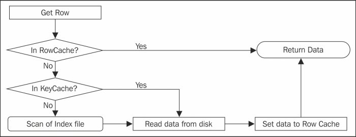
Row cache is true caching. It caches a complete row of data and returns immediately without touching the hard drive. It is fast and complete. Row cache stores data off-heap (if JNA is available), which means that it will be unaffected by the garbage collector.

Cassandra is capable of storing really large rows of data with about 2 billion columns in it. This means that the cache is going to take up much space, which may not be what you wanted. While row cache is generally good to boost the read speed, it is best suited for not-so-large rows. However, you can cache the users table in row cache, but it will be a bad idea to have the users_browsing_history or users_click_pattern table, in a row cache.

Key cache is to store the row keys in memory. Key caches are default for a table. It does not take much space, but it boosts performance to a large extent (but less than the row cache). As of Cassandra Version 2.1.0, the key cache is assigned to 100 MB or 5 percent of the JVM heap memory, whichever is low.

Key caches contain information about the location of the row in SSTables, so it's just one disk seek to retrieve the data. This short-circuits the process of looking through the sampled index and then scanning the index file for the key range. Since it does not take large space as row cache, one can have large number of keys cached in relatively small memory.

The general rule of thumb is, for all normal purposes, key cache is good enough. You can tweak key cache to stretch its limits. You'd get a lot of performance gain for just a little increase in key cache size in key cache settings. Row caching, on the other hand, needs a little thinking to do. A good fit data for row cache is the same as a good fit data for a third-party caching mechanism. The data should be read mostly, and mutated occasionally. Rows with smaller number of columns are better suited. Before you go ahead with cache tweaking, you may want to check the current cache usage. You can use JConsole to see cache hit. We will learn more about JConsole in Chapter 7, Monitoring. In JConsole, the cache statistics can be obtained by expanding the org.apache.cassandra.db menu. It shows cache hit rate and the number of hits and cache size for a particular node and table.

Cache settings are mostly global as of Version 2.1.0. The settings can be altered in cassandra.yaml. At table level, the only choices that you have are the cache type to use with or if you should use any cache at all. The options are: keys only, rows only, both and none. The following is an example (for more discussion, refer to the Creating a table section in Chapter 3, Effective CQL):

CREATE TABLE users (
user_id uuid,
email text,
password text,
PRIMARY KEY (user_id)
)
WITH
caching = {
'keys' : 'ALL',
'rows_per_partition' : '314'
};

The following are the caching-specific settings in cassandra.yaml:

The caches are saved under the directory that is described by the saved_caches_directory setting in the .yaml file. We configured it during the cluster deployment in Chapter 4, Deploying a Cluster. The default value for this setting is 14,400 seconds.

Table (or column family) compression is a very effective mechanism to improve read and write throughput. As one can expect, compression (any) leads to compact representation of data at the cost of some CPU cycles. Enabling compression on a table makes the disk representation of the data (SSTables) terse. This means efficient disk utilization, lesser I/O, and a little extra burden to the CPU. In the case of Cassandra, the trade-off between I/O and the CPU, due to compression, almost always yields favorable results. The cost of CPU performing compression and decompression is less than what it takes to read more data from the disk.

Compression setting is table-wise; if you do not mention any compression mechanism, LZ4Compressor is applied to the table by default. This is how you alter compression type (see details about assigning compression setting when the table is created in Chapter 3, Effective CQL):

ALTER TABLE users
WITH
COMPRESSION = {
  'sstable_compression': 'DeflateCompressor'
};

Let's see the compression options we have.

The sstable_compression parameter specifies which compressor is used to compress disk representation of SSTable, when MemTable is flushed (compression takes place at the time of flush). Cassandra Version 2.1.0 provides three compressors out of the box: LZ4Compressor, SnappyCompressor, and DeflateCompressor.

The LZ4Compressor is 50 percent faster than SnappyCompressor, which is faster than DeflateCompressor. In general, this means, when you move from DeflateCompressor to LZ4Compressor, the compression will take a little extra space, but it will have higher read speed.

Like everything else in Cassandra, compressors are pluggable. You can write your own compressor by implementing org.apache.cassandra.io.compress.ICompressor, compiling the compressor, and putting the .class or .jar files in the lib directory. Provide the fully-qualified class name of the compression as the sstable_compression value.

The chunk length (chunk_length_kb) is the smallest slice of the row that gets decompressed during reads. Depending on the query pattern and median size of the rows, this parameter can be tweaked in such a way that it is big enough to not have to deflate multiple chunks, but small enough to not have to decompress excessive unnecessary data. Practically, it is hard to guess this. The most common suggestion is to keep it 64 KB, if you do not have any idea.

Compression can be added, removed, or altered anytime during the lifetime of a table. In general, compression always boosts performance and it is a great way to maximize the utilization of disk space. Compression gives double to quadruple reduction in data size when compared to an uncompressed version. So, one should always set a compression to start with, and it can be disabled pretty easily as follows:

# Disable Compression
ALTER TABLE users
WITH
COMPRESSION = {
  'sstable_compression': ''
};

It must be noted that enabling compression may not immediately halve the space used by SSTables. The compression is applied to the SSTables that get created after the compression is enabled. With time, as compaction merges SSTables, older SSTables get compressed.

Accessing a disk is the most expensive task. Cassandra thinks twice before needing to read from a disk. The bloom filter helps to identify which SSTables may contain the row that the client has requested. Alternatively, the bloom filter being a probabilistic data structure, yields a false positive ratio (refer to Chapter 2, Cassandra Architecture). The more the false-positives, the more the SSTables needed to be read before realizing whether the row actually exists in the SSTable or not.

The false-positive ratio is basically the probability of getting a true value from the bloom filter of an SSTable for a key that does not exist in it. In simpler words, if the false-positive ratio is 0.5, chances are that 50 percent of the times you end up looking into the index file for the key but it is not there. So, why not set the false-positive ratio to zero; never make a disk touch without being 100 percent sure. Well, it comes with a cost—memory consumption. If you remember from Chapter 2, Cassandra Architecture, the smaller the size of the bloom filter, the smaller the memory consumption. A smaller bloom filter increases the likelihood of the collision of hashes, which means a higher false positive. So, as you decrease the false-positive value, your memory consumption shoots up. Therefore, we need a balance here.

In the bloom filter, the default value of the false-positive ratio is set to 0.000744. To disable the bloom filter, that is, to allow all the queries to SSTable—all false positive—this ratio needs to be set to 1.0. One may need to bypass the bloom filter by setting the false-positive ratio to 1, if one has to scan all SSTables for data mining or other analytical applications.

You can create a table with the false-positive chance as 0.001 as follows:

# Create column family with false positive chance = 0.001
CREATE TABLE toomanyrows (id int PRIMARY KEY, name text)
WITH
bloom_filter_fp_chance = 0.001;

One may alter the false-positive chance on an up-and-running cluster without any need to reboot. Alternatively, the false-positive chance is applied only to the newer SSTables—created by means of flush or via compaction.

One can always see the bloom filter chance by running the describe command in cqlsh or cassandra-cli or by running a nodetool request for cfstats. The node tool displays the current ratio too. The following is an example using the DESC command:

# Incassandra-cli
 DESC TABLE toomanyrows;
CREATE TABLE demo_cql.toomanyrows (
    id int PRIMARY KEY,
    name text
) WITH bloom_filter_fp_chance = 0.001
    [-- snip --]
    AND speculative_retry = '99.0PERCENTILE';

The current ratio is displayed via nodetool (all the statistics are zero because the table is unused, but as soon as you start reading and writing out of it statistics like this are pretty helpful to make decisions):

bin/nodetool cfstats demo_cql.toomanyrows
Keyspace: demo_cql
  Read Count: 0
  Read Latency: NaN ms.
  Write Count: 0
  Write Latency: NaN ms.
  Pending Flushes: 0
Table: toomanyrows
  SSTable count: 0
      [-- snip -- ]
  Bloom filter false positives: 0
  Bloom filter false ratio: 0.00000
  Bloom filter space used, bytes: 0
  [-- snip --]
    Compacted partition mean bytes: 0
    Average live cells per slice (last five minutes): 0.0
    Average tombstones per slice (last five minutes): 0.0

Durability—as we know from Chapter 2, Cassandra Architecture—provides durable writes by the virtue of appending the new writes to the commit logs. This is not entirely true. To guarantee that each write is made in such a manner that a hard reboot/crash does not wash off any data, it must be fsync'd to the disk. Flushing commit logs after each write is detrimental to write performance due to slow disk seeks. Instead of doing that, Cassandra periodically (by default, commitlog_sync: periodic) flushes the data to the disk after an interval described by commitlog_sync_period_in_ms in milliseconds. However, Cassandra does not wait for commit log to synchronize; it immediately acknowledges the write.

This means that if a heavy write is going on and the machine crashes, at the most, you will lose the data written in the commitlog_sync_period_in_ms window. You should not really worry. We have a replication factor and consistency level to help recover this loss; unless you are unlucky enough that all the replicas die in the same instant.

The commitlog_sync setting gives high performance at some risk. To someone who is paranoid about data loss, Cassandra provides a guarantee write option. Set commitlog_sync to batch mode. In batch mode, Cassandra accrues all the writes to go to the commit log, and then fsyncs after commitlog_sync_batch_window_in_ms, which is usually set smaller such as 50 milliseconds. This prevents the problem of flushing to the disk after every write, but the durability guarantee forces the acknowledgement (that the data is persisted) to be done only after the flush is done or the batch window is over, whichever is sooner. This means the batch modes will always be slower than the periodic modes.

For most practical cases, the default periodic value and default fsync() period of ten seconds will do just fine.

The column_index_size_in kb property tells Cassandra to add a column index if the size of a row (serialized size) grows beyond the KBs mentioned by this property. In other words, if row size is 314 KB and column_index_size_in_kb is set to 64 (KB), there will be a column index with at least five entries, each containing the start and the finish column name in the chunk and its offset and width.

If the row contains many columns (wide rows) or you have columns with really large-sized values, you may want to increase the default. It has a con; for a large column index in KB, Cassandra will need to read at least this much amount of data, even a single column of a small row with small values needs to be read. On the other hand, a small value for this property, large index data will need to be read at each access. The default is okay for most of the cases.

The commit log file is memory mapped (mmap). This means that the file takes the virtual address space. Cassandra flushes any unflushed MemTables that exist in the oldest memory mapped commit log segment to the disk. Thinking from the I/O point of view, it does not make sense to keep this property small because the total space of smaller commit logs will be filled up quickly, requiring frequent write to the disk and higher disk I/O. On the other hand, we do not want commit logs to hog all the memory. Note that the data that was not flushed to the disk. In the event of a shutdown, it is replayed from the commit log. So, the larger the commit log, the more the replay time it will take to restart.

The default for the 32-bit JVM is 32 MB and for 64-bit JVM is 1024 MB. You may tune it based on the memory availability on the node.

If you look at conf/cassandra-env.sh, you will see nicely written logic that does the following: max(min(1/2 ram, 1024MB)and min(1/4 ram, 8GB). This means that the max heap depends on the system's memory as Cassandra chooses a decent default, which is as follows:

The reason to not go down with a large heap is that garbage collection does not do well for more than 8 GB of RAM. A high heap may also lead to poor page cache of the underlying operating system. In general, the default serves good enough. If you choose to alter the heap size, you need to edit cassandra-env.sh and set MAX_HEAP_SIZE to the appropriate value.

Further down the cassandra-env.sh file, you may find the garbage collection setting as follows:

# GC tuning options
JVM_OPTS="$JVM_OPTS -XX:+UseParNewGC"
JVM_OPTS="$JVM_OPTS -XX:+UseConcMarkSweepGC"
JVM_OPTS="$JVM_OPTS -XX:+CMSParallelRemarkEnabled"
JVM_OPTS="$JVM_OPTS -XX:SurvivorRatio=8"
JVM_OPTS="$JVM_OPTS -XX:MaxTenuringThreshold=1"
JVM_OPTS="$JVM_OPTS -XX:CMSInitiatingOccupancyFraction=75"
JVM_OPTS="$JVM_OPTS -XX:+UseCMSInitiatingOccupancyOnly"
JVM_OPTS="$JVM_OPTS -XX:+UseTLAB"

Cassandra, by default, uses concurrent mark and sweep garbage collector (CMS GC). It performs garbage collection concurrently with the execution of Cassandra and pauses for a very short while. This is a good candidate for high-performance applications such as Cassandra. With the concurrent collector, a parallel version of the young generation copying collector is used. Thus, we have UseParNewGC, which is a parallel copy collector that copies surviving objects in young generation from Eden to Survivor spaces and from there to old generation. It is written to work with concurrent collectors such as CMS GC.

Further, CMSParallelRemarkEnabled reduces the pauses during the remark phase.

The other garbage settings do not impact garbage collection significantly. However, low values for CMSInitiatingOccupancyFraction may lead to frequent garbage collection because concurrent collection starts if the occupancy of the tenured generation grows above the initial occupancy. The CMSInitiatingOccupancyFraction option sets the percentage of current tenured generation size.

If you decide to debug the garbage collection, it is a good idea to use tools such as JConsole, in order to look into how frequent garbage collection takes place, CPU usage, and so on. You may also want to uncomment the GC logging options in cassandra-env.sh to see what's going on beneath the Cassandra process.

The other JVM options are as follows: