
In this chapter, I will pick up on one of the most popular use cases within banks that is migrating trade data from traditional relational data sources to Hadoop. This is also known as online data archiving. You are archiving your data to cheaper disks but are still be able to process the data.
In this chapter, I will cover the full data life cycle of the project:
- Data collection—collect data using shell commands and Sqoop
- Data analysis—analyze data using shell, Hive, and Pig
This chapter will be a little more technical with a few code templates, but I will try to keep it simple. I recommend you to refer to the Apache Hadoop documentation (http://hadoop.apache.org/), if you need to dive deeper.
When we acquire a new data warehouse in any financial organization, the fundamental design is based on this question, "What do we need to store and for how long?"
Ask this question to businesses and their answer will be simple—Everything and forever. Even regulatory requirements, such as Sarbanes-Oxley, MiFiD, and Dood-Frank Act, stipulate that we need to store records for at least 5 to 7 years and the data needs to be accessible in a reasonable amount of time. Today, that reasonable amount of time is not weeks, as before, but in the order of days or even one business day for certain types of data.
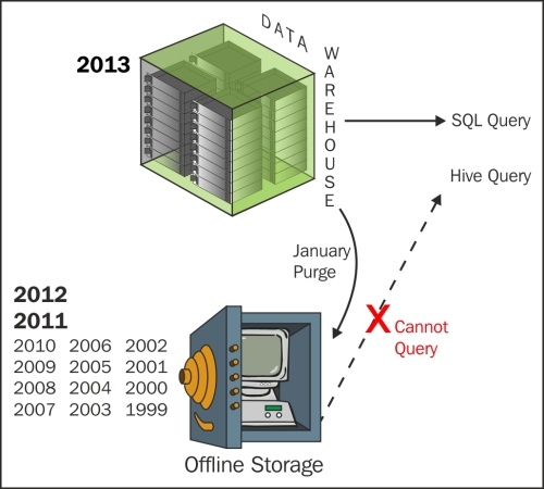
In banks, data warehouses are mostly built on high-performance enterprise databases with very expensive storage. So, they retain only recent data (say the last year) at the detailed level and summarize the remaining 5 to 10 years of transactions, positions, and events. They move older data to tapes or optical media to save cost. However, the big problem with this approach is as shown in following figure—the detailed data is not accessible unless it is restored back to the database, which again costs time and money:
The problem of storage is even worse, because generally the trade, event, and position tables have hundreds of columns on data warehouses.
In fact, business is mostly interested in 10–15 columns of these tables on a day-to-day basis and all other columns are rarely queried. But business still wants the flexibility to query less frequently used columns, if they need to.
Hadoop HDFS is a low-cost storage and has almost unlimited scalability and thus is an excellent solution for this use case. One can archive historical data from expensive high-performance databases to low-cost HDFS, and still process the data.
Because Hadoop can scale horizontally, simply by adding more data nodes, the business can store as much as they like. As you can see in the following figure, data is archived on Hadoop HDFS instead of tapes or optical media, which makes the data accessible quickly. This also offers flexibility to store less frequently used columns on HDFS.
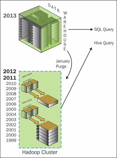
Once data is on HDFS, it can be accessed using Hive or Pig queries. Developers can also write MapReduce jobs for slightly more complicated data access operations.
Low-cost data warehouse online archives is one of the simplest Hadoop projects for banks to implement and has an almost immediate return on investment.
In this chapter, I will discuss a project to archive data into Hadoop in two phases:
- Phase 1: While loading transactions from source systems into a relational data warehouse, load frequently used columns into the data warehouse and all columns into HDFS
- Phase 2: Migrate all transactions that are older than a year from the relational data warehouse to HDFS
The incoming trade data that is currently loaded into the relational data warehouse will be split into two parts—frequently used business-critical data columns and a complete set of columns.
The critical data columns will be loaded into the relational data warehouse and a complete set of incoming data will simply be archived onto HDFS.
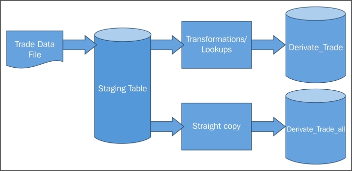
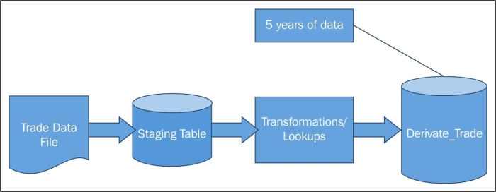
They receive the derivative trade as a very large file every night on the landing file server of a data warehouse system. The file is loaded into the staging table and subsequently into two very large data warehouse tables:
derivative_trade(the main derivative trade table with business-critical columns only)—stores 5 years of trade dataderivative_trade_all(derivative trade table with all columns, as the business hasn't explicitly defined which columns they need to access)—stores 1 year of trade data
The current data flow before Phase 1 implementation is shown in the following figure:
The derivative_trade table has 14 business-critical columns:
|
Trade Number Trade date Account Number Party ID Counterparty ID Business date Market |
Transaction Type Value date Buy Sell flag Quantity Price Total commission and fee Trade currency |
Even with 14 columns and millions of trades on a daily basis, the total database table size can easily run into terabytes within a year.
I will give you an example of a complete derivative transaction table structure (with 80+ columns) that is stored on many trade data warehouses. If you compare it with the main derivative_trade table with 14 columns, it shows how much data may be stored in the data warehouses without much benefit.
The complete transaction table derivative_trade_all looks as:
|
Premium Execution Type Open Close Flag LME Trade Type GiveIn Or GiveOut Trade Give Up Firm Cabinet Trade Type CTI Code Commission Rates Counterparty Commission Rates Commission Value Counterparty Commission Value Commission Currency Counterparty Commission Currency Tax Amount Counterparty Tax Amount Premium Held/Paid Flag Post Comms Upfront Flag Comm Override Flag EFP Cash Date Clearing Fee Suppress Clearing Fee Flag Clearing Fee Currency Exchange Fee Exchange Fee Currency Suppress Exchange Fee Flag NFA Fee Suppress NFA Fee Flag NFA Fee Currency Execution Charge Suppress Execution Fee Execution Fee Currency Fee Amount 5 Suppress Fee 5 Fee Flag Fee 5 Currency Give in Give Out Charges Suppress Give In Give Out Flag Give In Give Out Currency Brokerage Charge Suppress Brokerage Flag Brokerage Currency Other Charge Other Allocation Charges Suppress Other Allocation Charges Flag |
Suppress Other Charges Flag Other Charges Currency Fee Amount 6 Suppress Fee 6 Fee Flag Fee 6 Currency Back Office Charge Suppress Back Office Charge Flag Back Office Charge Currency Floor Charges Suppress Floor Charges Flag Floor Charges Currency Suppress Order Desk Charges Flag Other Allocation Charges Currency Order Desk Charges Order Desk Charges Currency Wire Charges Suppress Wire Charges Flag Wire Charges Currency Group Code 1 Group Code 2 Group Code 3 Group Code 4 Group Code 5 Group Code 6 Group Code 7 Group Code 8 Group Code 9 Group Code 10 Commission Currency Counterparty Commission Currency Clearing Fee Currency Exchange Fee Currency NFA Fee Currency Execution Fee Currency Fee 5 Currency Give In Give Out Currency Brokerage Currency Other Changes Currency Fee 6 Currency Back Office Charge Currency Floor Charges Currency Other Allocation Charges Currency Other Desk Charges Currency Wire Charges Currency |
With 88 columns and millions of trades on a daily basis, the total database table size can easily run into terabytes within just 3 to 4 months.
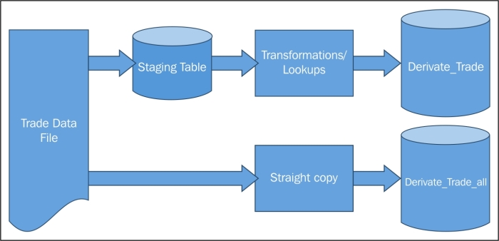
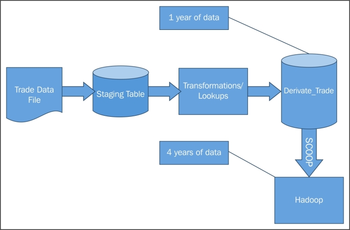
During the first phase of the project, they will continue to receive the derivative trade as a very large file every night on the landing file server of a data warehouse system and the file will still be loaded into the staging table and derivative_trade exactly the way it was before, but they will stop the existing load to the database derivative_trade_all and import the file from the landing server into Hadoop instead, saving them money in terms of database storage.
The data flow after Phase 1 implementation will look like the one shown in the following figure:
The data management on HDFS is very similar to shell commands. I will briefly cover certain configurations and assumptions:
- Configure the target location in HDFS. I recommend that you follow a good naming convention for the target directory, something as
<default_directory>/<system_name>/<purpose>/<file_or_table_name>. The system name can be something such astrade_dband the purpose can be something as archive or analytics. - I assume that the target location is
<default_directory>/trade_db/archive/derivative_trade_all. - You can use Putty or any other Linux SSH client to connect to the data warehouse landing file server and the Hadoop server.
- I assume all historical derivative files are archived on the file landing server.
Please follow these steps to archive the trade data to HDFS:
- Create a target location on HDFS using the following command:
hdfs dfs –mkdir <default_directory>/trade_db/archive/derivative_trade_all - Verify the target location on HDFS using this command:
hdfs dfs –ls <default_directory>/trade_db/archive/derivative_trade_all - Upload the file from the landing server to the target location on HDFS using the following command:
hdfs dfs –put <landing_server_directory>/derivative_file_all_<YYYMMDD>.txt <default_directory>/trade_db/archive/ derivative_trade_allYou can optionally use this:
hdfs dfs –copyFromLocal <landing_server_directory>/derivative_file_all_<YYYMMDD>.txt <default_directory>/trade_db/archive/derivative_trade_all/derivative_file_all_<YYYMMDD>.txt - Verify the target file on HDFS by running:
hdfs dfs –ls <default_directory>/trade_db/archive/ derivative_trade_all - If everything looks good, repeat this exercise for all the historical data files for one year.
- The daily load commands can be packaged as a script and scheduled.
- If you still miss your data-warehouse-type SQL, I recommend you to create an external Hive table. The external table is simply a mapping of the HDFS file with a Hive table. The command template to create a Hive table assumes the data file is comma delimited:
CREATE EXTERNAL TABLE IF NOT EXISTS derivative_trade_all (
Premium         FLOAT,
Execution_Type      STRING,
Open_Close_Flag      STRING,
LME_Trade_Type      STRING,
GiveIn_Or_GiveOut_Trade    STRING,
Give_Up_Firm      STRING,
Cabinet_Trade_Type    STRING,
CTI_Code        STRING,
…………………………….
Back_Office_Charge_Currency  STRING,
Floor_Charges_Currency    STRING,
Other_Allocation_Charges_Currency  STRING,
Other_Desk_Charges_Currency  STRING,
Wire_Charges_Currency    STRING)
ROW FORMAT DELIMITED FIELDS TERMINATED BY ','
LOCATION '<default_directory>/trade_db/archive/derivative_trade_all';
Once you have the data in Hadoop HDFS, it can be accessed in a variety of ways using Shell commands, Hive, or Pig, as described briefly in the following sections.
You can export the Hadoop file to your local landing server or desktop by downloading the file from Hadoop to the landing server, using the following command:
hdfs dfs –get <default_directory>/trade_db/archive/ derivative_trade_all/ derivative_trade_all_<YYYMMDD>.txt <landing_server_directory>/
You can optionally use this:
hdfs dfs –copyToLocal <default_directory>/trade_db/archive/ derivative_trade_all/derivative_file_all_<YYYMMDD>.txt <landing_server_directory>/derivative_file_all_<YYYMMDD>.txt
You can use most of the standard SQL commands you would have been using already when your data was on the relational data warehouse. For example:
- Select all records from the Hive external table (mapped to HDFS file) using the following command:
Select * from derivative_trade_all; - The table has 88 columns, so only select the columns you like, using this:
Select Premium, Execution_Type, Open_Close_Flag from derivative_trade_all; - Filter records using this command:
Select Premium, Execution_Type, Open_Close_Flag from derivative_trade_all where Premium > 10; - Group records by running:
Select Execution_Type, sum(Premium) from derivative_trade_all where Premium > 10 group by Execution_Type;
You can run Pig in local or MapReduce mode, depending on the environment. For development on a local installation, use local mode, or else use MapReduce mode.
- Use the following Pig commands to run in local or MapReduce mode:
/* local mode */
pig -x local ...
/* mapreduce mode */
pig ...
or
pig -x mapreduce ...
- Use the interactive mode to develop your scripts or for ad hoc queries or data operations. Simply invoke the Grunt shell using the following Pig command:
$ pig
... - Connecting to ...
grunt>
Pig statements are generally of three types:
- A
LOADstatement to read data from HDFS - A series of transformation statements to process the data
- A
DUMPstatement to view results interactively orSTOREstatement to save the results in a file
In our case, the command template will be as follows:
A = LOAD '<default_directory>/trade_db/archive/ derivative_trade_all/derivative_file_all_<YYYMMDD>.txt' USING PigStorage(',') AS
(Premium:float,
Execution_Type:chararray,
Open_Close_Flag:chararray,
LME_Trade_Type:chararray,
GiveIn_Or_GiveOut_Trade:chararray,
Give_Up_Firm:chararray,
Cabinet_Trade_Type:chararray,
CTI_Code:chararray,
…………………………….
-----------
Back_Office_Charge_Currency:chararray,
Floor_Charges_Currency:chararray,
Other_Allocation_Charges_Currency:chararray,
Other_Desk_Charges_Currency:chararray,
Wire_Charges_Currency:chararray);
B = FOREACH A GENERATE Premium;
DUMP B;
They have a relational table derivative_trade with millions of trades on a daily basis. The table has 5 years of data and takes up to 60 terabytes of storage (without adding further storage taken by indexes). The majority of reports and analytics require only the last 1 year's data. With the database storage almost 10 times more expensive than Hadoop storage, they will reduce storage costs and total cost of ownership (TCO) simply by migrating all data older than a year from the relational DW into Hadoop.
This phase of the project will migrate all transactions older than a year to Hadoop, followed by periodic monthly data moves to Hadoop.
They receive the derivative trade as a very large file every night on the landing file server, which then gets loaded into the staging table and then subsequently into the derivative_trade table. The main derivative trade table is the one with 14 business-critical columns and 5 years of trade data.
The current data flow before Phase 2 implementation is as shown in the following figure:
They will continue to receive the derivative trade as a very large file every night on the landing file server of a data warehouse system. The file will still be loaded into the staging table and derivative_trade exactly the way it was before, but now they have the additional task to migrate the older data from the derivative_trade table into Hadoop.
At the end of the migration, the table derivative_trade will only have 1 year of trade data and all the trades older than a year will be migrated to Hadoop.
The data flow after Phase 2 implementation will be as shown in the following figure:
The data is collected from the existing relational data warehouse (DW). You may have guessed already that the tool to migrate the data into Hadoop is Sqoop.
For this phase, I will make a few assumptions:
- Sqoop is already installed and configured on the Hadoop cluster.
- The database is a MS SQL Server and the server hostname is
trade_db. The JDBC drivers are installed, ready to be used by Hadoop. - The master trade table name is
derivative_trade, which has only the business-critical 14 columns, as shown here:Trade_number
Trade_date
Account_number
Party_id
Counterparty_id
Business_date
Market
Transaction_type
Value_date
Buy_sell_flag
Quantity
Price
Total_commission_and_fee
Trade_currency
Sqoop is a small utility with just a handful of commands and is therefore very easy to learn.
Simply type in the following command to get a list of all available commands:
sqoop help
Check the connection using the following command, which will list the available databases:
sqoop list-databases --connect jdbc:sqlserver://<DW IP Address>:Port --username <username> --password <password>
I recommend using a separate password file that has restricted access:
$ sqoop list-databases --connect jdbc:sqlserver://<DW IP Address>:Port --username <username> --password-file ${user.home}/.password
If you can see the database trade_db in the list of all available databases, move to the next step.
Now come the commands to import data into Hadoop.
If you need to know more on the syntax and all its arguments, simply type in the following command:
sqoop help import
For our exercise, I will list down some of the frequently used arguments and their value:
--connect <jdbc-uri>: JDBC connect string configured fortrade_dbdatabase.--password-file: Path for the file containing the authentication password with access-restricted permissions.-P: This argument will enable you to read the password from the console and should be used only during initial configuration or testing.--password <password>: This is the authentication password and should be used only during initial configuration or testing.--username <username>: This is the authentication username and should be used only during initial configuration or testing.--verbose: This argument will enable you to print more information while working and should be used during the development or test phases only.--append: Use this to append data to an existing dataset in HDFS.--columns <col,col,col…>: Use this to select columns to import from the tablederivative_trade. By default, all columns will be imported.--delete-target-dir: This argument is used to delete the import target directory if it exists and should be configured only for the initial data import, not periodic incremental imports.--fetch-size <n>: This is the number of entries to read from the database at once and it should be configured with the help of a DBA.--table <table-name>: This is the database table from which we will migrate the data to Hadoop. It isderivative_tradein our case.--target-dir <dir>: This is the HDFS destination directory; that is,<default directory>/trade_db/archive/derivative_trade.--where <where clause>: This is used to filter records from the database table during import.
You will need to first migrate all database records older than a year into Hadoop using a where clause (--where parameter) with a condition such as WHERE TRADE_DATE < CURRENT_DATE – 1 YEAR. In MS SQL Server, it will be something as:
WHERE TRADE_DATE < DateAdd(yy, -1, GetDate())
Once the initial data has been loaded into HDFS and the successful verification of the data has been completed using Hive or Pig queries, the data from derivative_trade on the data warehouse can be deleted using the following:
Delete from derivative_trade WHERE TRADE_DATE < DateAdd(yy, -1, GetDate())
It is likely that the database tables will be partitioned by date or months. If that is the case, simply query those explicit partitions and drop the table partitions, once it has been migrated into Hadoop.
You need to create and schedule a script, which will load incremental data from derivative_trade into Hadoop.
Sqoop's incremental import command has a few additional arguments, they are as follows:
--check-column (col): This specifies the column to determine which rows to import. It cannot be text or string. In this case, it will betrade_date.--incremental (mode): This specifies how Sqoop determines which rows are new; the valid values are append and last modified. You should specify the append mode when importing a table where new rows are continually being added with increasing row ID values. Specify the last modified mode when rows of the source table may be updated with the current timestamp.--last-value (value): This specifies the maximum value of the check column from the previous import.
Once the incremental data has been successfully migrated to Hadoop, delete the data that has been migrated from derivative_trade. It is highly possible that the data will be partitioned by date or month. I recommend the periodic incremental migration frequency to be in sync with the data partitions, for better performance.
Instead of only importing the data into HDFS, Sqoop can directly import data from the relational database to Hive's internal tables.
For this exercise, the relevant command is again import, but the arguments are slightly different, compared to when importing into HDFS:
--hive-import: Use this argument to import tables into Hive (Hive's default delimiters will be used if none are specified)--hive-overwrite: This argument will overwrite existing data in the Hive table and should therefore be used carefully--hive-table <table-name>: This will set the table name in Hive and I recommend you to use the same table name as in the relational data warehouse, if you intend to reuse some of your existing SQL queries
Hive will have problems if you are using Sqoop-imported data when your database's rows contain string fields with Hive's default row delimiters (
and
characters) or column delimiters (�1 characters). You need to use the --hive-drop-import-delims option to drop those characters during import to give Hive-compatible text data.
Alternatively, you can also use the --hive-delims-replacement option to replace those characters with a string of your choice during import to give Hive-compatible text data. These options should only be used if you use Hive's default delimiters, and should not be used if other delimiters are specified.
Sqoop also provides you the option to load the relational trade data into HBase for real-time queries. In this case of migration, there is no such requirement to load it into HBase. But feel free to explore it if there is any such requirement.