
5
Exteroceptive Fault-tolerant Control for Autonomous and Safe Driving
5.1. Introduction
In recent decades, the pace at which technological advances have become available has sharply accelerated. In the last 30 years, the personal computer, the Internet, mobile networks as well as many other innovations have transformed human lives. Beyond science fiction-like visions, we have searched for substitutes for repetitive, physically challenging tasks, replacing them with machines or robots reaching beyond human capabilities or with computer programs under the supervision of human beings. Among these machines, the automobile has revolutionized the daily transport of millions of people and the number of cars has grown steadily since the democratization of the vehicle. This explosion of the number of cars gave rise to many problems, such as traffic jams, air pollution due to greenhouse gases and soil pollution associated with liquid and solid discharges (motor oils and heavy metals). Accidents are still one of the biggest road-related problems. The annual report of the French Road Safety Observatory (L'observatoire national interministériel de la sécurité routière – ONISR), estimated for 2015 [ONS 16], revealed that the number of deaths related to road traffic accidents had increased by 1.7% in comparison with the previous year, producing a total of 3,616 fatalities. Even though this number is lower compared to the 1980s, it is still unacceptable. At the global scale, more than 1.25 million people die in road accidents. The question then points to the main causes of these accidents and invites us to find the obstacles we should tackle in order to reduce the number of road accidents. In fact, the analysis of accident technique [ONS 16] revealed that the driver still represents the main cause of accidents: speed represents 32% of accidents (main or secondary), driving under the influence of alcohol causes 21% of accidents and illegal drugs cause 9% of accidents. Lack of attention, dangerous overtaking, sleepiness, lane changing and sickness accounted for 31% of the cause of accidents. Vehicle factors accounted for only 1% of accidents.
Table 5.1. Main causes of accidents in France in 2015 (source: ONSIR) – the total represents 122% since multi-causes were considered
| Identified causes in a fatal accident | Percentage |
| Speed | 32% |
| Alcohol | 21% |
| Priority not given | 13% |
| Other causes | 12% |
| Illegal drugs | 9% |
| Unknown cause | 9% |
| Lack of attention | 7% |
| Dangerous overtaking | 4% |
| Sickness | 3% |
| Sleepiness or fatigue | 3% |
| Contraflow driving | 2% |
| Lane changing | 2% |
| Obstacles | 2% |
| Vehicle factors | 1% |
| Telephone use | 1% |
| No safe distance from previous vehicle | 1% |
| Total | 122% |
The causes of accidents were not the same for all age groups. In fact, novices and seniors mostly made mistakes related to not giving priority. On the other hand, alcohol and speed were the causes of the majority of accidents among younger people. The rates of accident causality per age group are shown on the histogram in Figure 5.1.

Figure 5.1. Statistics on causes of accidents by age group (source: ONSIR). For a color version of this figure, see: www.iste.co.uk/vanderhaegen/automation.zip
An accident is rarely triggered by a single cause: it is actually a conjunction of several causes, of which speed is often the aggravating factor. For example, driving under the influence of illegal drugs may induce high speed and lack of attention, followed by dangerous overtaking. That being said, the human factor was still the main cause for the majority of road traffic accidents in France in 2015. In fact, humans have to perform a variety of actions while driving: they have to perceive the environment, analyze and understand it, adopt and outline a driving strategy and carry it out through actuators. Tiredness, distraction, miscalculation, unconsciousness, etc. may provoke mistakes in each of these actions and eventually lead to accidents. In addition to road safety, fuel consumption is a concern for the human driver. In addition, Barth and Boriboonsoms in [BAR 09] proved that adopting an eco-driving system could help save between 10% and 20% of fuel. On another note, this economic process could help reduce the emission of carbon dioxide and nitrogen oxides into the atmosphere and thereby reduce atmospheric pollution. [BOU 10, HAJ 10].
In order to respond to these challenges, researchers and engineers have introduced various advanced driver-assistance systems (ADAS). This may explain the design of active safety systems, such as the collision avoidance system [HAL 01] and the lane departure warning system [JUN 04], in order to avoid accidents, or intelligent speed monitoring systems, with the aim of optimizing fuel consumption, as introduced by [BAR 08, AKH 16], or reducing risk on road curves [GLA 10, GAL 13]. However, active security systems struggle to achieve the expected results, due to the fact that they are limited to specific cases, and the interaction of these systems with the driver is still problematic and ambiguous. In fact, several recent incidents have been caused by a misunderstanding between human and machine, or at least by the latter’s limitations. Such technical limitations basically concern navigation systems, which may display non-existent sections of road, which is what happened to an American driver who was using the Waze app and found himself crossing a frozen lake, before the ice broke [AFP 18].
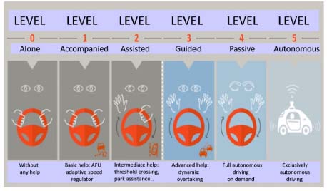
Figure 5.2. Vehicle automation levels (source: Argus)
Automated driving seems to provide a global solution for the problems described above. Ideally, for an automated vehicle, every task involving perception, localization, planning and control should be executed by sensors, algorithms and actuators [JO 14], only allowing the driver to choose the destination to be reached. Based on this principle, several autonomous vehicle projects worldwide are going through the research phase, such as Google’s GoogleCar/Waymo. Others are interested in specific operation areas, such as Renault’s or General Motor’s prototypes. The goal is to achieve a high level of automation (i.e. level 4 or 5 according to the definition by SAE International [SAE 16], as shown in Figure 5.2), considering the driver as a fallback solution during failure scenarios or operating within specific environments (level 4), or in every possible situation (level 5), by providing autonomous monitoring of the vehicle’s environment, the performance of its sensors and algorithms, and the action to be taken in order to keep the vehicle in a safe state. The task of automation seems difficult to accomplish, given the wide range of road scenarios to consider, and the vehicle should be able to react to any damage, and especially to failures in its own means of perception. The diagnosis is therefore an essential step for detecting and isolating sensor faults as soon as these appear, in order to enable stable and safe driving, enhanced by fault-tolerant control. In this chapter, we will introduce a diagram of fault-tolerant control architecture based on voting algorithms so as to diagnose the faults of exteroceptive sensors.
This chapter is organized as follows: a formulation of the problem is illustrated in section 5.2; section 5.3 is devoted to the architecture of fault-tolerant control; voting algorithms are detailed in section 5.4; section 5.5 shows the results of digital simulation and a conclusion is reached in section 5.6.
5.2. Formulation of the problem
Given the diversity of situations and problems that a vehicle may encounter, this chapter will focus on the problem of having to regulate inter-vehicle distance. Nevertheless, the real problem in measuring the inter-vehicle distance lies in the inability of technologies to properly operate in all working modes. The use of several sensor technologies helps to overcome each sensor’s limitation, by merging data. However, data fusion may be affected if the sensors have hardware or software faults, which may lead to erroneous measurements. Therefore, it is necessary to manage the reliability of these measurements and to ensure fault tolerance, in order to guarantee safe operation in autonomous mode [MAR 09].
This topic was partly addressed in [MAR 09], where the authors suggested a simple switching strategy to choose between three control loops, each consisting of a given sensor (radar, lidar and a camera), a condition observer and a controller. The switching mechanism chooses the control loop that minimizes a quadratic criterion, from those that can be found in a robust, fault-free invariant set. However, this method shows the disadvantage of being restrictive in the case of longitudinal tracking, since it does not take into account the orientation of the front vehicle. In [REA 15, REA 16], multi-sensor fusion architecture was introduced, minimizing the influence of sensor faults. This technique was based on a fusion structure controlled by an SVM (Support Vector Machine) module for detecting faults. The fault detection block compared the divergences between the outputs in:
- – two local fusion structures, each using a Velodyne sensor and a vision sensor;
- – a master fusion structure.
The Velodyne sensor is considered as a reference sensor in both local fusion structures. Also, the data from the fusion are based on the weights generated by the SVM block. The purpose of this technique is to ensure that, were an obstacle to be detected, it would be possible to measure the distance between the obstacle and the autonomous vehicle. The disadvantage of this method lies in the fact that it employs cascade detectors, which may increase calculation time.
In this context, the purpose of our contribution is to suggest an approach based on voting algorithms so as to reduce the impact of sensor faults and to ensure safe autonomous driving. This method has been widely used for approaching fault tolerance problems. In fact, this technique has been broadly applied in the field of engineering, thanks to the ease of its design and its implementation. It has been applied in many areas such as graphology [ONA 16], medical monitoring [GAL 15], electric vehicles [BOU 13, RAI 16, SHA 17] and aeronautics [KAS 14].
5.3. Fault-tolerant control architecture
In order to ensure its reliability, the autonomous vehicle is equipped with three sensor technologies that may be used for longitudinal control: a long-range radar, a lidar and a Mobileye smart camera, which calculates the distance. Each of these sensors has a specific limitation, and does not work at its best under certain circumstances. For example, as the lidar is based on sending and receiving spectrum light waves, it can lead to aberrant detections in bad weather, such as in the presence of fog, heavy rain or dust particles.
In addition, the lidar cannot detect color or contrast, and does not guarantee a good identification of the nature of the objects. On the other hand, the radar may not detect the vehicle ahead, due to the difference in speed between the leading and following vehicles. The radar may also be unable to detect motorcyclists or other vehicles ahead when they are outside the center of the lane. In addition, the smart camera may not work thoroughly if the lens is partially or completely obstructed. The latter does not guarantee a 100% rate of detection of the vehicle ahead. In this way, weather conditions greatly influence the recognition and response capabilities of the smart camera.
As we mentioned earlier, each sensor has limitations that mainly depend on the technology employed and its operating area. Each sensor may be faulty in its operating area due to a software or hardware failure, leading to erroneous distance measurement. In order to solve these malfunctions, fault-tolerant control should manage all possible scenarios and keep autonomous driving stable and safe, as shown in Figure 5.3. Voting algorithms are intended to diagnose the faulty sensor by making a comparison between healthy signals, with the aim of ensuring stable and safe driving.

Figure 5.3. Fault-tolerant control architecture, based on voting algorithms
The monitoring speed is set by the reference speed generating block. The latter is deduced from the safety distance relation, resulting from the following relation [TOU 08]:
Then, from equation [5.1], we can deduce the reference speed as follows:
where dstop represents the distance to be respected at the stop and h represents the inter-vehicle time (usually between one second and three seconds).
5.3.1. Vehicle dynamics modeling
Vehicle dynamics is known for being very complex and strongly interconnected. In order to illustrate the dynamics governing the behavior of a vehicle, it is necessary to resort to a number of simplifying assumptions, so as to reduce the model’s complexity [HED 97, BOU 17b]:
- –only one fault per sensor will be considered;
- –the road will be supposed to be flat (with no slopes, no inclination);
- –the lateral dynamics of the vehicle will not be taken into consideration;
- –rolling, lacing and pitching movements will not be taken into account.
Considering the assumptions made, the longitudinal dynamics of the vehicle can be expressed as follows:

When adopting a bicycle model [HED 97, BOU 17a]:

We obtain the following equation:

By substituting Fxf and Fxr in equation [5.3], we get:

| Notation | Definition | Unit |
| m | Mass of the vehicle | kg |
| Vx | Vehicle speed | ms–1 |
| Fxi | ith wheel–ground contact force | N |
| Fa | Aerodynamic force | N |
| Overall inertia of the front axle | kgm2 | |
| Inertia of the ith front wheel | kgm2 | |
| Angular acceleration of the ith wheel | rad.s–1 | |
| Tm | Engine coupler | Nm |
| r | Wheel radius | m |
| Fri | Rolling friction of the ith wheel | N |
| Tbi | Braking torque of the ith wheel | Nm |
| T rf/r | Rolling resistance: front vs. rear axle | Nm |
| Jri | Inertia of the ith rear wheel | kgm2 |
| Jr | Overall inertia of the rear axle | kgm2 |
Also, let us assume that the wheels do not slip throughout the maneuver. This assumption can be interpreted by the following equation:
which leads to rωr = Vx, and then ![]() .
.
Replacing ![]() in equation [5.5], we obtain:
in equation [5.5], we obtain:
We then adopt the following notation:
Equation [5.6] becomes:
where: ![]() , and a as well as b are aerodynamic coefficients. Teq represents the braking and accelerating torque. In order to overcome the delay problem related to the dynamics of braking and accelerating, we will assume that the accelerating/braking pair is governed by a first-order equation, written as follows:
, and a as well as b are aerodynamic coefficients. Teq represents the braking and accelerating torque. In order to overcome the delay problem related to the dynamics of braking and accelerating, we will assume that the accelerating/braking pair is governed by a first-order equation, written as follows:
Finally, the longitudinal dynamics of the vehicle is expressed by the following relation [PHA 97]:

5.4. Voting algorithms
As shown in Figure 5.3, a voting algorithm is able to choose a safe distance measure only by using sensor measurement signals. This distance is obtained by comparing the signals produced by the sensor/processing units, after which the voting logic chooses the most reliable signal. The voting techniques used for this task are: maximum likelihood, weighted averages and history-based weighted average.
5.4.1. Maximum likelihood voting (MLV)
The first work on MLV was published in [LEU 95]. The basic idea of this approach is to choose one of the input signals, ensuring the highest probability in terms of reliability. Thus, for each dynamic reliability dedicated to the sensors written as fi, with i = 1,2,………N, where N represents the number of sensors, conditional probabilities Δi are calculated based on the equation below [KIM 96, RAI 16]:
In our case study, we use three sensors (intelligent camera, radar and lidar), so N = 3. Dmax is a fixed real number, corresponding to the threshold (this is fixed at 10% of the reference range in order to apprehend the effect of noise on the voting algorithm), where xk is the reference input.
The probability of each input sensor is calculated by the following formula:

The output signal is then chosen in such a way that it satisfies the maximum likelihood:
5.4.2. Weighted averages (WA)
The weighted averages method is based on the weight coefficients attributed to each sensor. Therefore, the output of the algorithm represents the average of the measured signals. Furthermore, the output signal is determined as a continuous function of the redundant inputs when we use weighted averages. In fact, this technique aims to reduce the transitory effect, in such a way that no switching is allowed, and the faulty sensor is isolated, with zero weight attributed to it (or a minimal weight, in the practical case) [BRO 75]. Therefore, considering an input signal xi, with i = 1,2 … … … N, where N is the number of sensors, the output signal y is determined by the following equation:
where wi, with i = 1,2, … … … N, are the weight coefficients. These coefficients correspond to the sum of the inverse distances of all input signals compared to the others, so that if the signals are close to the others, it implies a high weight.

In addition, the weight is obtained as follows:
where Ki j are the inverse of the distances between the input signals, which are represented by:
5.4.3. History-based weighted average (HBWA)
The underlying idea of this technique is to use a history that informs about the state of the sensors. Indeed, over time, a reliability index is accumulated for each sensor, so that the sensor that is chosen at the output of the algorithm has the highest reliability. Latif-Shabgahi, Bass and Bennett [LAT 01] presented two philosophies for this technique. The first one, called agreement state indicator weighted average, employs a dynamic weighting function based on the indicator’s status. Then, the weights are proportionally related to the indicator history. The second method, called module elimination weighted average, calculates an average of the indicator’s history, and then every entry with an historic indicator below this average is considered unreliable; therefore, its weight is set to zero. The HBWA technique is based on the algorithm introduced below:
- 1) For input signals xi and xj, coefficients kij are calculated in the following form:
where i, j = 1,2,… … …N and i≠j.
- 2) Using adjustable threshold parameters a and q, the agreement level for each input is given by:

- 3) The level of consensus Si calculated as:
- 4) The wi weighting for input i is calculated in the following form:
where Pi(n) and Pavg(n) are the indicators of the ith sensor’s status in the nth calculation cycle and the average of the indicating status in the nth calculation cycle, respectively. These will be discussed later.
- 5) An initial output, denoted as
 , is then calculated using the input signals of sensor xi and weights wi:
where i = 1,2,… … … N.
- 6) The distances between the initial output signal and the input signal for each sensor are calculated in order to determine the appropriate final output:
where i = 1,2, … … … N.
- 7) The final output y is expressed by the following equation:
- 8) The history H(n) of the ith sensor is recorded in the nth voting cycle, calculating the consensus h(n) level of the current cycle, based on the distance between each sensor xi and the final output y:

Thereafter, the history is given by:
- 9) The Pi(n) status indicator of the ith input in the nth voting cycle is calculated by the following equation:
- 10) Finally, the indicator of Pavg(n) average status, in the nth voting cycle, is determined as follows:

5.5. Simulation results
In this section, we will introduce the simulation results obtained from our fault-tolerant control architecture. The first step is to determine the MLV and HBWA threshold parameters. In order to achieve this, we employ an iterative method based on extended simulation. The threshold values are given as follows: a = 0.007, q = 700 and Dmax = 1.37. Each sensor has a variable reliability with regards to its operating range.
On the other hand, the reliability of each sensor technology differs. Thus, the lidar is reputed to be more reliable than the other two, and its reliability is not affected by a variation regarding the obstacle’s distance. Also, the reliability of the lidar is fixed at fLidar = 99%, whereas the radar is more reliable over long distances when the reliability relationship fRadar = 0.00067.d + 0.95 is respected. The smart camera has better precision over short distances with an expression of reliability equal to fcamera = - 0.0013.d + 0.97.
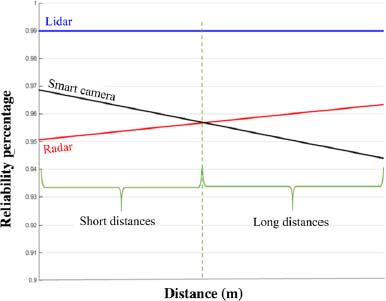
Figure 5.8. Reliability variation depending on the distance, according to three different sensor technologies
For this simulation, we adopted a scenario of following a leading vehicle while respecting a safety distance relative to the speed of the autonomous vehicle. This scenario is schematically illustrated in Figure 5.3. Thus, the leading vehicle starts at a speed of 20 m/s, and keeps it constant until t = 25 s. The autonomous vehicle initially drives at a speed of 25 m/s and quickly stabilizes and maintains 20 m/s in order to respect the safety distance of formula [5.2]. At t = 25 s, the leading vehicle rapidly puts on the brakes and reaches zero speed at t = 33 s, then remaining at rest.

Figure 5.9. Fault emulation on different sensor measurements. For a color version of this figure, see: www.iste.co.uk/vanderhaegen/automation.zip


Figure 5.11. Inter-vehicle distance using the maximum likelihood voting (MLV) algorithm. For a color version of this figure, see: www.iste.co.uk/vanderhaegen/automation.zip

Figure 5.12. Sensor transition using the maximum likelihood voting (MLV) algorithm
By regulating the inter-vehicle distance, the autonomous vehicle also quickly puts the brakes on until it stops. When the cars are stopped, the distance between the leading vehicle and the autonomous vehicle is equal to 3 m, that is, distance dstop defined in formula [5.2]; in our case, this stopping distance is considered when it reaches 3 m. At t = 40 s, the leading vehicle initiates an acceleration and becomes stable at a speed of 20 m/s until = 60 s, before putting on the brakes, in order to reach zero speed at t = 65 s and maintain its standstill until = 75 s, when the leading vehicle re-accelerates and reaches a speed of 12 m/s. As a result, the autonomous vehicle regulates and adapts its speed in accordance with that of the leader, always keeping a suitable safety distance.
In order to separately test the voting algorithms developed in section 5.4, we will emulate faults occurring on exteroceptive sensors (lidar, radar and camera). Figure 5.9 represents the emulation of faults on sensors, which are often associated with complete failures producing null signals. Also, the faults on sensors are emulated at moments t = [7 s 13 s] for the radar, t = [64 s 74 s] for the camera and t = [35 s 41 s [∪] 130 s 170 s] for the lidar.
In order to ensure a certain tolerance to the faults injected, the purpose of the voting algorithms is to detect the faulty sensor, choosing the most reliable measurement. Thus, the generated reference speed will be the most representative of reality, which would maximize the safety of the controlled vehicle.
The first algorithm we tested is that of maximum likelihood. Figure 5.11 shows the output of the MLV algorithm compared to the actual inter-vehicle distance (reference distance). The output of the MLV algorithm seems to provide a perfect picture of the true distance between the two vehicles (with a detection rate and an error rate for each sensor), the faults emulated on the sensors having been eliminated. This is related to the fact that the voting logic always chooses the most reliable sensor within the chosen distance range. Thus, Figure 5.12 shows the transitions between sensors at the output algorithm. Moreover, as the lidar has the best reliability, it will always be preferred over the others. However, as soon as this fails, the algorithm will choose the most reliable sensor depending on the range of distance measured. Therefore, the algorithm chooses the camera at t = [35 s 41 s], because the distance is short and the camera is more reliable in this case, whereas at t = [130 s 170 s], the algorithm chooses the radar, because the radar is more suitable at this distance.

Figure 5.13. Inter-vehicle distance using the weighted averages (WA) algorithm. For a color version of this figure, see: www.iste.co.uk/vanderhaegen/automation.zip
For the second algorithm, the algorithm’s output compared to the reference distance (actual distance) is shown in Figure 5.13. The output of the WA algorithm seems to deviate a little from the actual distance. Such deviation may be explained by the fact that this algorithm offers an output weighted by the coefficients it calculates from sensor inputs. Thus, the output represents a fusion between the three signals admitted at the input. In addition, if we consider the evolution of the weights of the three sensors shown in Figure 5.14, then we will note that the weights do not completely disappear when the sensor fails, which influences the result offered by the algorithm. In addition, even when all the sensors are working under normal operating conditions, the weighting calculation mechanism favors the sensors providing the closest results, which can be detrimental to the proper functioning of the algorithm.

Figure 5.14. Weights of the weighted averages (WA) algorithm. For a color version of this figure, see: www.iste.co.uk/vanderhaegen/automation.zip
Unlike the WA algorithm, the history-based weighted average algorithm offers a much better result. The output of the HBWA algorithm is shown in Figure 5.15, where we can reckon that it accurately represents inter-vehicle distance.

Figure 5.15. Inter-vehicle distance using the history-based weighted average (HBWA) algorithm. For a color version of this figure, see: www.iste.co.uk/vanderhaegen/automation.zip

Figure 5.16. Evolution of state indicators (HBWA). For a color version of this figure, see: www.iste.co.uk/vanderhaegen/automation.zip
By keeping a record of the state of each sensor (Figure 5.16), this technique favors the sensor which has worked under normal operating conditions (without failure) for the longest time, and contrary to the weighted averages (WA), where the output is an average of the three inputs, the HBWA algorithm chooses one sensor among three. This choice responds to the limitation set by the history, as well as by the closest sensor to a weighted average of the three sensors.
A comparison of the algorithm’s output inter-vehicle distance between the three voting techniques is shown in Figure 5.17, where we can note a clear advantage of the MLV and HBWA techniques over the WA technique, whereas there is a slight difference between the first two. The latter is still the most powerful algorithm, as long as it can provide a proper image of each sensor’s reliability. On the other hand, since the reference speed (the comparison in Figure 5.18) is directly calculated from the output inter-vehicle distance of voting algorithms, we can note the same appearance for the speed reference profile as for that of the inter-vehicle distance. This proves the dependence of the generation of the reference speed on the proper functioning of the voting algorithm.
The dynamic performance of the autonomous vehicle is also dependent on the performance of the algorithms, as we can infer from the comparison of the speed (Figure 5.19) and acceleration (Figure 5.20) profiles. The strong variations in the reference speed of the WA and the smaller variations of the MLV are clearly visible on the speed profile. These variations in speed influence the acceleration, even though this is still considered acceptable for the case studied.

Figure 5.17. Comparison of inter-vehicle distance using the three algorithms. For a color version of this figure, see: www.iste.co.uk/vanderhaegen/automation.zip

Figure 5.18. Reference speed comparison. For a color version of this figure, see: www.iste.co.uk/vanderhaegen/automation.zip

Figure 5.19. Speed profile comparison. For a color version of this figure, see: www.iste.co.uk/vanderhaegen/automation.zip

Figure 5.20. Acceleration profile comparison. For a color version of this figure, see: www.iste.co.uk/vanderhaegen/automation.zip
5.6. Conclusion
Accident statistics on roads point to the human factor as one of the major causes. As a solution, replacing the driver in relation to different driving actions seems appropriate both in terms of accidentology and other societal problems, such as transport-related pollution, by optimizing consumption. Nonetheless, this requires sensor technologies that deliver robust and reliable information in relation to the variety of situations that a vehicle may come upon. In order to remedy the problem of exteroceptive sensor faults in the case of longitudinal autonomous driving, a comparative study of three voting algorithms (MLV, WA and HBWA) was featured. In fact, this approach proved its capacity and efficiency in the diagnosis of faulty sensors. In addition, the history-based weighted average (HBWA) algorithm offered better performance than the other two algorithms. The efficient performance of the HBWA algorithm is derived from the fact that it chooses one sensor among three, making sure that the selected sensor has not experienced failure on previous occasions. This ability represents a significant advantage in comparison with the MLV, which makes an immediate switch as soon as the fault appears. On the other hand, the setting of threshold parameters for MLV and HBWA is still difficult to obtain due to the chattering effect. On the other hand, the operating range must be properly studied because a fixed threshold cannot grant a good performance along a wide range of operation.
The results presented in this study have shown that voting algorithms can ensure fault tolerance for autonomous vehicles. Indeed, the ability to diagnose faulty sensors in order to use other sensors will ensure a safe and stable trajectory for an autonomous vehicle, as it will maximize safety for human passengers. On the one hand, the simplicity of the design and of the implementation of voting algorithms can guarantee this capability. On the other hand, these algorithms do not require much calculation time to identify faulty sensors, which makes us privilege them over data fusion, which requires a great amount of calculation time.
5.7. References
[AFP 18] AFP, “États-Unis : ils suivent Waze et terminent dans un lac”, Le Parisien avec AFP, January 25, 2018.
[AKH 16] AKHEGAONKAR S., NOUVELIÉRE L., GLASER S. et al., “Smart and green ACC: energy and safety optimization strategies for EVs”, IEEE Transactions on Systems, Man, and Cybernetics: Systems, vol. 48, no. 1, pp. 142–153, 2016.
[BAR 08] BARBÉ J., BOY G., “Analysis and modelling methods for the design and evaluation of an eco-driving system”, Proceedings of European Conference on Human Centred Design for Intelligent Transport Systems, 2008.
[BAR 09] BARTH M., BORIBOONSOMSIN K., “Energy and emissions impacts of a freeway-based dynamic eco-driving system”, Transportation Research Part D: Transport and Environment, vol. 14, no. 6, pp. 400–410, 2009.
[BOU 10] BOUKHNIFER M., HAJ SALEM H., “Évaluation opérationnelle de la régulation d’accès sur les autoroutes de l’IDF basée sur la stratégie ALINEA”, IEEE Conférence internationale francophone d’automatique (CIFA’10), Nancy, June 2–4, 2010.
[BOU 13] BOUKHNIFER M., RAISEMCHE A., DIALLO D. et al., “Fault tolerant control to mechanical sensor failures for induction motor drive: a comparative study of voting algorithms”, 39th Annual Conference of the IEEE Industrial Electronics Society (IECON 2013), pp. 2851–2856, 2013.
[BOU 17a] BOUKHARI M.R., CHAIBET A., BOUKHNIFER M., “Fault tolerant design for auto-nomous vehicle”, 4th International Conference on “Control, Decision and Information Technologies” (CoDIT), pp. 721–728, 2017.
[BOU 17b] BOUKHARI M.R., CHAIBET A., BOUKHNIFER M. et al., “Fault-tolerant control for Lipschitz nonlinear systems: vehicle inter-distance control application”, IFAC-PapersOnLine, vol. 50, no. 1, pp. 14248–14253, 2017.
[BRO 75] BROEN R., “New voters for redundant systems”, Journal of Dynamic Systems, Measurement, and Control, vol. 97, no. 1, pp. 41–45, 1975.
[GAL 13] GALLEN R., HAUTIERE N., CORD A. et al., “Supporting drivers in keeping safe speed in adverse weather conditions by mitigating the risk level”, IEEE Transactions on Intelligent Transportation Systems, vol. 14, no. 4, pp. 1558–1571, 2013.
[GAL 15] GALEOTTI L., SCULLY C.G., VICENTE J. et al., “Robust algorithm to locate heart beats from multiple physiological waveforms by individual signal detector voting”, Physiological Measurement, vol. 36, no. 8, pp. 1705–1716, 2015.
[GLA 10] GLASER S., MAMMAR S., SENTOUH C., “Integrated driver-vehicle-infrastructure road departure warning unit”, IEEE Transactions on Vehicular Technology, vol. 59, no. 6, pp. 2757–2771, 2010.
[HAJ 10] HAJ SALEM H., BOUKHNIFER M., MABROUK H. et al., “Le contrôle d’accès généralisé sur les autoroutes de l’Île-de-France : études en simulation et sur site réel”, 8th IFAC International Conference of Modeling and Simulation – MOSIM’10, Hammamet,
May 10–12, 2010.
[HAL 01] HALL B.O., Collision avoidance system, Patent no. 6223125B1, 2001.
[HED 97] HEDRICK J.K., GERDES J.C., MACIUCA D.B. et al., Brake system modeling, control and integrated brake/throttle switching: phase I, Research report, California Partners for Advanced Transit and Highways (PATH) Institute of Transportation Studies, 1997.
[JO 14] JO K., KIM J., KIM D. et al., “Development of autonomous car – part I: distributed system architecture and development process”, IEEE Transactions on Industrial Electronics, vol. 61, no. 12, pp. 7131–7140, 2014.
[JUN 04] JUNG C.R., KELBER C.R., “A lane departure warning system based on a linear-parabolic lane model”, Intelligent Vehicles Symposium IEEE, pp. 891–895, 2004.
[KAS 14] KASSAB M., TAHA H., SHEDIED S. et al., “A novel voting algorithm for redundant aircraft sensors”, 11th World Congress on Intelligent Control and Automation (WCICA), pp. 3741–3746, 2014.
[KIM 96] KIM K., VOUK M.A., MCALLISTER D.F., “An empirical evaluation of maximum likelihood voting in failure correlation conditions”, 7th International Symposium on Software Reliability Engineering, pp. 330–339, 1996.
[LAT 01] LATIF-SHABGAHI G., BASS J.M., BENNETT S., “History-based weighted average voter: a novel software voting algorithm for fault-tolerant computer systems”, 9th Euro-micro Workshop on Parallel and Distributed Processing, pp. 402–409, 2001.
[LEU 95] LEUNG Y.-W., “Maximum likelihood voting for fault-tolerant software with finite output-space”, IEEE Transactions on Reliability, vol. 44, no. 3, pp. 419–427, 1995.
[MAR 09] MARTÍNEZ J.J., SERON M.M., DEDONÁ J.A., “Multi-sensor longitudinal control with fault tolerant guarantees”, IEEE European Control Conference (ECC), pp. 4235–4240, 2009.
[ONA 16] ONAN A., KORUKOGLU S., BULUT H., “A multi objective weighted voting ensemble classifier based on differential evolution algorithm for text sentiment classification”, Expert Systems with Applications, vol. 62, pp. 1–16, 2016.
[ONS 16] ONSIR, La sécurité routière en France, Bilan de l’accidentalité de l’année 2015, 2016.
[PHA 97] PHAM H., TOMIZUKA M., HEDRICK J.K., Integrated maneuvering control for automated highway systems based on a magnetic reference/sensing system, Research Report, California Partners for Advanced Transit and Highways (PATH), Institute of Transportation Studies, UC Berkeley, 1997.
[RAI 16] RAISEMCHE A., BOUKHNIFER M., DIALLO D., “New fault-tolerant control architectures based on voting algorithms for electric vehicle induction motor drive”, Transactions of the Institute of Measurement and Control, vol. 38, no. 9, pp. 1120–1135, 2016.
[REA 15] REALPE M., VINTIMILLA B., VLACIC L., “Sensor fault detection and diagnosis for autonomous vehicles”, MATEC Web of Conferences, no. 30, 2015.
[REA 16] REALPE M., VINTIMILLA B., VLACIC L., “Multi-sensor fusion module in a fault tolerant perception system for autonomous vehicles”, 2nd International Conference on Robotics and Artificial Intelligence, Los Angeles, 2016.
[SAE 16] SAE, “Taxonomy and definitions for terms related to driving automation systems for on-road motor vehicles”, available at: doi.org/10.4271/J3016_201609, 2016.
[SHA 17] SHAO J., DENG Z., GU Y., “Fault-tolerant control of position signals for switched reluctance motor drives”, IEEE Transactions on Industry Applications, vol. 53, no. 3, pp. 2959–2966, 2017.
[TOU 08] TOULOTTE P.-F., DELPRAT S., GUERRA T.-M. et al., “Vehicle spacing control using robust fuzzy control with pole placement in LMI region”, Engineering Applications of Artificial Intelligence, vol. 21, no. 5, pp. 756–768, 2008.
Chapter written by Mohamed Riad BOUKHARI, Ahmed CHAIBET, Moussa BOUKHNIFER and Sébastien GLASER.