
3
The Universe and the Earth
Contemporary of Newton, Leibniz, and French mathematicians René Descartes (1596–1650) and Pierre de Fermat (1607–1665), Blaise Pascal (Figure 3.1) embodied an ideal form of all of them: that of a knowledgeable man. A physicist, mathematician and philosopher, he evoked, in one of his most famous texts, the singular place of humanity on Earth and in the Universe:
“Let humanity therefore contemplate the whole of nature in its high and full majesty, let us keep our sight away from the low objects that surround us. Let us look at this bright light put like an eternal lamp to illuminate the Universe, let the earth appear to us as a point at the cost of the vast tower that this star describes and let us be surprised that this vast tower itself is only a very delicate point towards the one that these stars, which roll in the firmament, embrace” ([PAS 60], translated from French).
Are researchers in astrophysics and geophysics, in the 21st Century, the heirs of the 17th Century scientists? With numerical simulation, they nowadays carry out real thought experiments, supported by data, in fields where concrete experimentation is not easily accessible – or even simply possible.
Solving certain enigmas of the Universe, which extend Pascal’s philosophical observations, and contributing to the analysis of geophysical risks – in order not to reduce it to a probability calculation – are two areas in which numerical simulation is becoming increasingly important.

Figure 3.1. Blaise Pascal (1623–1662)
COMMENT ON FIGURE 3.1.– Early inventor of a computing machine (Chapter 4 of the first volume), Blaise Pascal was passionate about physics and mathematics. He was interested in the notion of vacuum, experimented with the laws of fluid hydrostatics and laid the foundations for the calculation of probabilities. His mystical experience turned him from science to theology: his ambition was to write a treatise on it, of which Les Pensées, found after his death, are the working notes (source: Blaise Pascal, anonymous, 17th Century, oil on canvas, Château de Versailles).
3.1. Astrophysics
An orchestral explosion punctuated by the percussion of timpani inaugurates the Representation of Chaos. It slowly fades into a long decrescendo ending in a marked silence. In a tiny pianissimo, an uncertain sound world is then born, whose tonality only gradually asserts itself. Through contrasting and apparently erratic episodes, ranging from the imperceptible murmur to the brutal explosion, the overture to The Creation, written by Austrian composer Joseph Haydn (1732–1809), then subsides into a transition giving Raphael the floor. The latter describes, in a short recitative, the world as “formless and empty” of the “dark abyss”. In a pianissimo breath, the choir entered in turn by evoking “the spirit of God” and proclaimed fortissimo “let there be light!” He is accompanied by the entire orchestra, supporting his song to a chord of D Major, powerful, radiant and luminous! Uriel concludes with a very short recitative of the introduction to this oratorio: “And God saw that the light was good… God separated the light from the darkness”. First performed in Vienna in 1799, this musical work begins with the first three minutes of the Universe. It seems to anticipate by more than a century the Big Bang theory, an idea supported in the 1930s by the observations of the American astronomer Edwin Hubble (1889–1953).
The quest for the origin of the Universe – as well as its possible future – has been built by improving the theoretical knowledge and sensitivity of observational instruments over time. Astrophysicists studying the Universe, its formation and evolution, nowadays have an additional tool at their disposal: computer simulations. Patrick Hennebelle, a researcher at the CEA, at the Institute of Fundamental Laws of the Universe, explains:
“For more than twenty years, astrophysics has been taking advantage of numerical simulations. They allow us to understand and predict the behavior of certain celestial bodies and are applied in many fields: star physics, galaxy dynamics, planet formation or the evolution of the gaseous interstellar medium, etc. Simulations make it possible to reproduce astronomical observations, which involve the interaction of systems with highly variable densities, covering a very wide range, typically from 1 to 1010 particles per cm3! The models take into account electromagnetic forces, gravitational force and current research aim to better account for radiation processes, which are still poorly described in some simulations”.
Scientific computation also offers researchers the possibility of reproducing evolutionary sequences that cannot be understood in their entirety by other means, because they take place over several billion years! It is also a means of optimizing the use of the most modern astronomical observation resources (Figure 3.2). The latter are shared within an international community and their access, subject to calls for projects examined by expert commissions, is very competitive. Simulation allows researchers to prepare an observation sequence, by testing different hypotheses in advance, and can also be used to interpret the results.
Numerical models are becoming widespread in all disciplines of astrophysics, particularly the most advanced ones, contributing to the description of black holes and the search for gravitational waves, whose recent discovery is also due to modeling techniques (Box 3.1).

Figure 3.2. ALMA is an international astronomical observation tool, a network of 64 antennas installed in Chile
(source: © European Southern Observatory/C. Malin/www.eso.org)
3.1.1. Telling the story of the Universe
Our Universe was born some 13 billion years ago and the matter of which it is composed has been sculpted by the action of different fundamental physical forces. While the first few seconds of the Universe are still an enigma to cosmologists, its subsequent evolution is better known. Current physical models explain how the first particles (electrons, protons, neutrons – and beyond, elementary particles they are made of) and atoms (hydrogen and its isotopes, and then the range of known chemical elements) are formed under the influence of nuclear and electromagnetic forces (Figure 3.3). The history of the Universe is therefore that of a long aggregation of its matter that sees the formation of the first stars and galaxies and other celestial bodies (clusters and superclusters of galaxies). This organization is, among other things, the result of gravitational force.
The latter is described by Newton’s formula that some astrophysicists use to understand the structure of the Universe. In 2017, for example, researchers conducted one of the most accurate simulations to date of a piece of the Universe, using a so-called “N-body model” [POT 17]. The latter describes the gravitational interaction between a very large number of celestial bodies: the problem posed has no explicit mathematical solution and only a numerical method is able to give one. Romain Teyssier, one of the researchers behind this simulation, explains:
“This is a description of the gravitational forces acting on a large set of particles. They are of different sizes, and they represent celestial bodies: stars, star clusters, small or large galaxies (dwarfs or supernova), galaxy clusters, etc.”

Figure 3.3. A summarizing history of the Universe. For a color version of this figure, see www.iste.co.uk/sigrist/simulation2.zip
COMMENT ON FIGURE 3.3.– This illustration summarizes the history of our Universe, which spans almost 14 billion years. It shows the main events that occurred in the first eras of cosmic life, when its physical properties are almost uniform and marked by very small fluctuations. The “modern history” of the Universe begins some 1 to 10 million years after the Big Bang, from the moment it is dense enough for the gravitational force to orchestrate its global organization. It is marked by a wide variety of celestial structures: stars, planets, galaxies and galaxy clusters. Long considered as the “start” of the history of the Universe, the Big Bang became for modern physicists the marker of a transition between two states of the Universe. The question of the origin of the Universe remains open [KLE 14] (source: ©European Space Agency/C. Carreau/www.esa.int).
The simulation figures are, strictly speaking, astronomical. In order to achieve it, scientists use a square digital box, one side of which measures 3 billion parsec1.
The calculation box contains 2 trillion particles (2 million million or 2 thousand billion). It allows us to represent galaxies 10 times smaller than our Milky Way, which corresponds, for example, to the star cluster of the Large Magellanic Cloud. The simulation thus involves some 25 billion galaxies, whose evolution is observed over nearly 12.5 billion years and it is carried out in just under 100 h of computation.
On the day of the simulation, this resolution is considered very satisfactory by astronomers and astrophysicists. The calculation represents the places where matter has organized itself in the Universe under the influence of gravity (Figure 3.4) and provides data that are sufficiently accurate to be compared with observations made on the cosmos within a few years. Until now, the calculations did not have the accuracy required for this comparison to be relevant.
The simulation is made possible through two innovations:
- – The use of particularly efficient algorithms to model a very large number of particles. Directly simulating the interactions between N particles requires N2 operations: for the 2 trillion particles required for simulation, the amount of calculations to be performed is inaccessible to computers, even the most powerful ones! An appropriate method, known as the “fast multipolar method”, considerably reduces the number of calculation operations. It consists of representing the interactions of one particle with others by means of a tree, where the direct approach represents it by means of a network (Figure 3.5). In the tree, the interaction between the particles i and k is represented by the one they have with the particle j. By exploring the tree more or less deeply, we find all the interactions described by the network. Exploring the tree requires N operations, while the network one requires N2 operations. Under these conditions, the calculation at 2 trillion particles becomes possible. The validation of the simulation is obtained by comparing a direct calculation and an optimized calculation on a sample of a few million particles. The simulation describing the 2 trillion particles is then performed with the optimized algorithm.

Figure 3.4. Simulation of the state of the Universe organized under gravitational forces between celestial bodies
(source: Joachim Stadel, University of Zurich)

Figure 3.5. Interactions between particles can be described with a network or tree
- – The use of supercomputers that exploit the processing capacity offered by graphics cards (GPUs). Note that 5,000 graphics cards were simultaneously used on the supercomputer of the Swiss National Supercomputing Centre (Chapter 3 of the first volume), whose performance and architecture are currently unique in the world. The 100 hours of computing time required for simulation is entirely appropriate to the pace of the researchers’ work. By comparison, the duration of a parallel calculation on the same number of conventional processors (CPUs) is estimated by researchers at 20 years.
So, the calculation code is the result of a development work of about 20 years and its adaptation to the specificities of this simulation took about 3 years. Porting the algorithm to other supercomputers should allow for simulations with 10 or 100 times more particles, thus offering calculations a higher resolution.
3.1.2. Observing the formation of celestial bodies
The gravitational field plays an important role in the formation of black holes, and in order to understand the dynamics of these structures observed in the Universe and certain complex phenomena such as instabilities, researchers propose different physical and numerical models. The simulation then becomes a digital observatory to test many ideas or hypotheses explaining observations.
Some of the physics at play in the dynamics of celestial bodies (such as planets or black holes) is that of plasmas, a state of matter made up of charged particles. It may be described by the equations of magneto-hydro-dynamics (MHD), which express the conservation of the mass, momentum and energy of particles, on the one hand, and the propagation of electromagnetic waves within the plasma, on the other hand.
Two examples of simulations are proposed for the Rossby3 wave instability (Figure 3.15):
- – the first (top) corresponds to the evolution of a black hole and uses a calculation code developed by astrophysicists to study an instability evolving very quickly, in a few seconds;
- – the second (bottom) reproduces the formation mechanism of the heart of a planet, governed by similar physical mechanisms developing this time on longer time scales.
From the simulations, astrophysicists develop radiation spectra: a curve of light that indicates the presence of a black hole – or any other entity studied. Compared to spectra from celestial observations, they allow researchers to propose explanations of the observed phenomena and to test their validity.

Figure 3.15. Examples of simulation in astrophysics
To observe the formation of a planet’s core, the simulated physical time is a few million years and requires one month of calculation. The evolution of instabilities is significant over several hundred simulated years. The calculation must reproduce them and, in order to be reliable, not artificially generate them, which happens when digital schemas are not totally conservative. In such a case, the calculation may introduce numerical errors whose effect is to pollute the simulation. The simulated quantities are tainted with errors that produce oscillations, without any physical meaning.
In order to validate the calculation method – and to ensure the stability of the numerical schemas – a simulation is started in a neutral initial state, free of disturbance. It is a matter of ensuring that this state does not change. The energy signal emitted by the plasma is then zero over the entire duration of the simulation: in the absence of an external effect, absolutely nothing happens and this is what is desired. If the numerical scheme is conservative, then the calculation method can be used to see the plasma evolve under the effect of physical phenomena, only contained in the equations – and not induced by numerical calculation errors. This is an issue that is also found in many other industrial applications.
3.1.3. Predicting the mass of stars
Stars play a fundamental role in our Universe. They synthesize elements essential to certain life forms (carbon, oxygen, iron, etc.) and they contribute to the in-depth renewal of the composition of galaxies throughout their lives. They emit light energy necessary for certain chemical reactions to occur and, during explosions marking the end of activity of the largest ones, they emit a large quantity of matter into the Universe. The properties of stars vary with their mass:
- – High-mass stars have a “hot” temperature, their lifespan is relatively short (on the scale of the Universe!): up to a few tens of millions of years. Marked by intense energy activity, they burn gases by injecting turbulence into the Universe and contributing to its radiation.
- – Low-mass stars, like our Sun, have a “cold” temperature. Long-lasting, they contribute to the stability of planetary systems and generally host planets – potential life-bearers!
The distribution of the mass of the different stars makes it possible, among other things, to understand the history and functioning of the Universe. From observations of the cosmos (Figure 3.17), the distribution curve shows, for example, that the most frequent mass of stars is about one-third of the solar mass (denoted 0.3 Mo). It decreases quite quickly below (to the lower masses) and beyond (to the larger masses).

Figure 3.17. Stellar density map of our galaxy. For a color version of this figure, see www.iste.co.uk/sigrist/simulation2.zip
COMMENT ON FIGURE 3.17.– Created in 2018 by the European Space Agency using data from the “Gaia “ mission, the image represents a three-dimensional map of the stars observed in our galaxy, representing the most massive ones, which are also the warmest and brightest. The latter are mainly located near their training site, in the heart of the Milky Way. Regions of high stellar density are represented in pink and purple, intermediate density regions in violet and light blue, and low-density regions in dark blue. The map also shows areas of high concentrations of stardust, in green, and known clouds of ionized gas are identified by brown spheres. The map lists nearly 400,000 stars over a distance of 10,000 light-years from the Sun. Centered around the latter, the map represents the galactic disc observed from a point very far from our galaxy. With a database of the positions and trajectories of more than a billion celestial bodies, the “Gaia” mission is one of the most prolific to date, providing astronomers with detailed information (source:© European Space Agency/K. Jardin/www.esa.int).
This distribution seems to change very little from one part of the galaxy to another, and even from one galaxy to another, while physical conditions, such as density, can vary considerably. Patrick Hennebelle used numerical simulation (Figure 3.18) to understand the origin of this distribution, while studying the case of the stellar cloud:
“We have performed a series of calculations describing the dynamics of a collapsing stellar cloud of a thousand solar masses. By varying over large amplitudes, from 10 to 10,000 for example, different model parameters, such as density or turbulence intensity in the initial state of the cloud, or by modifying the laws of gas thermodynamics, we have studied numerous evolution scenarios and identified which physical parameters influence the dynamics of the stellar cloud”.

Figure 3.18. Stellar density calculations in a star cloud [LEE 17a]. For a color version of this figure, see www.iste.co.uk/sigrist/simulation2.zip
COMMENT ON FIGURE 3.18.– The figure represents the density of stars calculated in a collapsing cloud. It is represented in color by increasing values from blue (low density) to green (high density). The red dots mark stars of different masses whose formation is observed during the calculation (source: © CEA-DAp).
The result of the simulations first of all surprised the researcher, as the analysis of the calculations showed that thermodynamic phenomena explain the distribution observed on the masses of the stars. The gas state equation describes the radiation transfer processes that occur in the collapsing cloud; it controls the cooling of the gas, including its ability to remove excess gravitational energy. By varying the parameters of this equation, researchers have better understood the dynamics of the collapsing cloud.
“My initial idea was that thermodynamics played a minor role and we made this discovery almost by chance! The simulations then helped us in interpreting the results and developing a theory to explain them”.
The mechanism proposed after the analysis of the simulations predicts the correct value of the characteristic mass of the stars: it effectively leads to a stellar mass distribution in accordance with the observations (Figure 3.19).

Figure 3.19. Stellar density calculations [LEE 17b]. For a color version of this figure, see www.iste.co.uk/sigrist/simulation2.zip
COMMENT ON FIGURE 3.19.– The graph shows the distribution of stars produced in the collapse of a cloud according to their mass and under different assumptions introduced in the simulations. The distribution of the mass of stars has a maximum value around a mass of one-tenth of the solar mass, close to that observed in the cosmos (source: © CEA-DAp).
If simulation nowadays allows discoveries in astrophysics, it is difficult to attribute the sole merit to it:
“The calculations allow virtual experiments for which two questions are asked: the validation and understanding of the physical phenomena at work in the observed systems. A discovery involves a chain as a whole: observations, simulations and their interpretations”.
Simulation, which now plays an essential role in the development of knowledge in astrophysics, benefits from the advances of many digital disciplines: HPC computing techniques and AI algorithms are making their way into the astrophysicists’ toolbox [VAR 19]. In addition, some calculation methods originally developed by astrophysicists have more or less direct applications in the industry. This is the case with the so-called “SPH method”, for example, a particulate method initially invented to describe certain celestial dynamics. It is also used by engineers to solve flow equations under conditions where conventional methods encounter difficulties (Figures 2.1, 2.19 and 3.20).
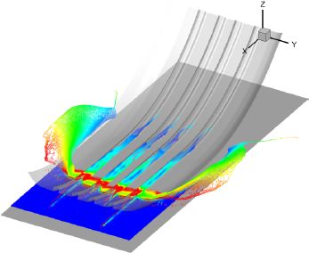
Figure 3.20. Aquaplaning simulation [HEM 17]. For a color version of this figure, see www.iste.co.uk/sigrist/simulation2.zip
COMMENT ON FIGURE 3.20.– This aquaplaning simulation helps to improve vehicle handling. The difficulty of the calculation lies in modeling the contact of the tyre on the road, which pinches a fluid blade. Most of the methods used for fluid mechanics simulations fail to reproduce aquaplaning. Based on the description of particles, the SPH method, initially developed to conduct astrophysical calculations, proves to be adapted to this situation.
3.2. Geophysics
Journey to the Center of the Earth is the third adventure novel published by Jules Verne [VER 64]. He recounts a scientific discovery – that of the depths of our planet, coupled with an initiatory adventure, that of the narrator of the story, the young researcher Axel Lidenbrock, who accompanies his uncle in his underground research – and emerges from this extraordinary experience. The novel was written at a time when geology was in full development. Extrapolating on the knowledge of his time, Verne’s imagination describes an Earth full of mineralogical and paleontological wonders (Figure 3.21): eternal diamonds, mushrooms or petrified trees, fantastic creatures – all species extinct from the surface of the globe (algae, fish or prehistoric monsters).

Figure 3.21. Illustration of Journey to the Center of the Earth [VER 64], plate no. 30, drawing by Édouard Riou (1833–1900)
(source: www.commons.wikimedia.org)
Advances in geophysics at the beginning of the 20th Century made it possible in particular to draw up a map of the Earth’s crust that was more in line with reality, highlighting its dynamic nature. The theory of plate tectonics was validated by the international scientific community in the 1960s. It explains the constant movements of the Earth’s mantle, which cause earthquakes, eruptions and tsunamis in various parts of the world. Responsible for terrible human losses, as well as very significant material damage, these events have left their mark on humans and their places of life for many years to come.

Figure 3.22. Age of the oceanic lithosphere [MUL 11]. For a color version of this figure, see www.iste.co.uk/sigrist/simulation2.zip
COMMENT ON FIGURE 3.22.– The colors on the map represent the age of the ocean lithosphere. The most recent zones, formed at the level of oceanic faults, are indicated in red. The age of the oldest areas (represented in purple) is estimated at 280 million years. The areas in green correspond to an average age of 130 million years. The black lines represent the boundaries of the tectonic plates. The movement speeds of the plates are in the order of a few centimeters per year. The fastest movements, about 20 cm/year, are recorded in some regions of Southeast Asia – such as Papua New Guinea – and the Pacific – such as the Tonga-Kermadec archipelago (source: https://www.ngdc.noaa.gov).
Over the past decade, digital simulation has become a widely used tool in geophysical sciences. Used by researchers in this discipline, it helps in the assessment of natural disasters risks. In the following, we will examine three fields of application: earthquakes, tsunamis and eruptions.
3.2.1. Earthquakes
Italy is located in an area of intense seismic activity: the life of the geological layers of this region is surrounded by the Alps to the northwest and by Mount Etna to the southeast of the country, which are evidence of tectonic activity. Characterized by violent ground movements, with acceleration levels far exceeding the acceleration of gravity, an earthquake is perceptible in all three spatial directions and produces strong mechanical stresses on buildings, often leading to their destruction. On Monday, April 6, 2009 at 3:52 am, the country experienced a major earthquake near L’Aquila, a town in the mountainous region of Abruzzo. With a magnitude of 6.2, its human toll was terrible: more than 300 dead and 1,500 wounded. The earthquake also destroyed many villages: about 40,000 buildings were demolished or severely damaged, affecting the lives of more than 70,000 people in the region. It is one of the most violent earthquakes recorded in Italy (Figure 3.23).

Figure 3.23. Recent seismic history of Italy (source: Emanuele Casarotti, National Institute of Geophysics and Volcanology). For a color version of this figure, see www.iste.co.uk/sigrist/simulation2.zip
COMMENT ON FIGURE 3.23.– The map shows earthquake records in Italy, classified by magnitude. This magnitude, representing the logarithmic energy released by an earthquake, is related to the damage it causes. A magnitude increase of 1 corresponds to a 30-fold increase in seismic energy.
A chain of solidarity was set up after this disaster: providing relief, shelter, care and comfort. For the rescuers, a race against time is underway. The aim is to search for possible survivors in the rubble as soon as possible. Hours of work without sleep, in very difficult conditions – and let us not forget: this is a Western country, rich and organized, with extensive human and technical resources.
In the case of such disasters, an additional danger comes from very strong aftershocks that can occur in the following days, on the same geological fault or on other faults located in the region. These aftershocks may endanger the lives of rescuers and people working in the debris. On Thursday, April 9, 2009, a very strong aftershock, magnitude 5.1, occurred and completed the destruction or damage of buildings in the L’Aquila region. Fortunately, residents had been evacuated from the heavily affected area since the first earthquake and the aftershock only caused material damage.
In a discreet way, a geophysics researcher and numerical simulation expert helped to assess the risk of this eventuality by locating potentially dangerous ground vibrations. It was carried out using numerical simulations of possible aftershocks from the initial earthquake.
After the first seismic tremors, seismologists gained accurate data on the disaster – for example, the coordinates of the epicenter of the earthquake as well as its approximate depth, and the accelerations recorded at different locations. They also became aware of the other geological faults in the impacted region and can speculate on how the original fault, or even others in the region, could fail. Dimitri Komatitsch tells us:
“In the aftermath of the L’Aquila earthquake, I was contacted by seismologists from the National Institute of Geophysics and Volcanology (INGV) in Rome to build a numerical model of the region concerned. Using a calculation code that a community developed over the years to simulate ground vibrations in the event of an earthquake, I built such a model in less than 12 hours, feeding it with geological data from the L’Aquila region and INGV data on the first earthquake”.
The calculations, sent to the Italian authorities for analysis, made it possible to obtain in a few hours the results of several aftershock hypotheses in the region for the days following the initial earthquake (Figure 3.24). The aftershock shown on the image was calculated in 2009. On 30 October 2016, the region experienced a seismic event whose global characteristics (magnitude, location of the epicenter and nature of the geological fractures) were very close to this calculation.

Figure 3.24. Scenario for the L’Aquila earthquake aftershock: in yellow and red, the areas potentially affected (source: calculations were carried out in 2009 by Dimitri Komatitsch at the Centre National de la Recherche Scientifique in France and Emanuele Casarotti at the National Institute of Geophysics and Volcanology in Italy). For a color version of this figure, see www.iste.co.uk/sigrist/simulation2.zip.
Second, the partial erasure of the aftereffects of such a disaster is slow. Before reconstruction, an inventory of damaged buildings must be logged (Figure 3.25) and safe repair options must be sought. For some residents, it takes years to return to normal life.

Figure 3.25. Traces of the earthquake on buildings in L’Aquila
(source: ©Alain Breyer/www.alainbreyer.be)
In order to use simulation in emergency situations, it is crucial to perform fast and accurate seismic aftershock calculations and the code used by the researcher has two advantages:
- – a particularly efficient calculation method solves the equation of seismic wave propagation in geological layers. These are described by means of a viscoelastic behavioral law [TRO 08]. This equation, also discussed in Chapter 1 of the first volume, is similar to that used for the vibration of musical instruments. It yields accurate results for large-scale seismic models (that of a given region);
- – the computing power of a supercomputer, at the time a partition of nearly 500 computing cores of a machine, assigned urgently for these life-size calculations by GENCI in France. The development choices made on the seismic simulation code at the time of its development made it particularly suitable for porting to HPC computing means [KOM 11].
The improvement of this seismic calculation tool remains at the heart of geophysicists’ research today:
“One of the main areas of development is a more detailed characterization of the basements. It is accomplished through seismic imaging, by comparing data recorded in situ after an earthquake and calculations made in these situations. The difference between the seismicity data recorded and their simulation allows for the iterative correction of geological layer models. To do this, the calculation codes constantly perform simulations: there are sometimes thousands of them for correcting a particular problem!”.
Simulations obviously do not make it possible to predict the date of the seismic event, its location or its intensity. They contribute to the production of probable data for risk analysis. As a reminder, a few days before the major earthquake, a commission of Italian experts met in L’Aquila to analyze a series of earthquakes that had occurred in the region in the previous months. While they were obviously unable to predict the imminent arrival of a stronger earthquake, they made recommendations on the potential dangers facing the region at that time. For some Italian citizens, these were insufficient. After the earthquake, the seven scientists on this commission were found guilty of negligence in their seismic risk analysis. They were accused of giving too much reassuring information to the population, who could have taken measures to protect themselves. The experts were sentenced to prison terms and acquitted 2 years later on appeal. These trials have had a strong impact on the families of the victims of the earthquake and have also caused a great deal of misunderstanding and emotion in the international scientific community. These facts raise questions about the place and role of scientists in the prevention of natural risks, and about citizens’ expectations of experts and even the sciences. Legitimate in the obligation of means and in the search for proven errors, such as negligence or breaches of mandatory and legal procedures, these expectations can sometimes be disproportionate, even unrealistic, given the current capacity of science and scientists to predict with certainty certain events and their effects. This capacity often remains limited, as in the case of seismic risk:
“The only current earthquake prevention measure is to identify areas at risk (L’Aquila was one), build buildings seismically (designed to withstand earthquakes) and educate people to take shelter at the very beginning of seismic movements…”5
Let us conclude this section by noting that the Earth shakes under the effect of tectonic movements as it also can under the effect of crowds –with a vibration energy that is nevertheless much lower [SIM 18]. During the 2018 football world cup, the vibrations generated by the jumps of joy of Mexican fans were recorded by the seismographs of the Mexican Atmospheric and Geological Research Institute6.
3.2.2. Tsunamis
Hokusai, master of Japanese printmaking, was nearly 70 years old when he published his 36 Views of Mount Fuji in 1830. His sumptuous images are a true worship of the sacred mountain: it is present in an imposing way, or by becoming more discreet, in all the landscapes or scenes of life that the artist represents there. The first print in the series is probably Hokusai’s best-known print. The Great Wave [CLA 11] testifies to Japan’s ancestral vulnerability to tsunamis.
On March 11, 2011 at 2:45 am, an earthquake of magnitude 9.0 occurred 130 km (81 miles) off the coast of Sendaï on Hinsu, the main island of the Japanese archipelago. This earthquake was the most devastating in Japan after the Kobe earthquake in 1995 (5,500 deaths). It was the fourth most intense earthquake ever recorded since the first measuring devices were deployed in 1900. The tsunami caused was the deadliest since the Hokkaido tsunami in 1993 (200 deaths).
Images of the country’s devastation and the pain of its inhabitants left their mark on the entire world. The official report drawn up in February 2015 by the Japanese authorities indicated that 15,890 people were killed and 2,590 missing or presumed dead, as well as 6,152 injured in the country’s 12 prefectures. The earthquake and tsunami caused nearly $220 billion in damage in Japan and contributed to the disaster at the Fukushima I (Daiichi) nuclear power plant – with severe consequences for the health of the country’s population and economy.

Figure 3.26. An underwater earthquake can cause a tsunami (source: © www.shuterstock.com). For a color version of this figure, see www.iste.co.uk/sigrist/simulation2.zip
COMMENT ON FIGURE 3.26.– A tsunami is a train of ocean waves generated by seabed movements, themselves resulting from an earthquake or eruption. At high depths, the tsunami wave has a very small amplitude in the order of a few centimeters. When it arrives near the coast, it can take on a much greater amplitude and break into a turbulent wall several meters high.
The effects of the tsunami were felt throughout the Pacific Rim. It caused damage estimated at nearly $30 million on the island of Hawaii, destroying U.S. Navy facilities, and caused more than $6 million in losses to the fishing industry in the city of Tongoy, Chile – more than 16,000 km from the epicenter of the earthquake. Satellite observations also revealed for the first time the effects of the tsunami on the collapse of the Antarctic ice cap.
The prevention of such disasters is based, among other things, on an observation of the state of the seas. In the Pacific Ocean, the DART (Deep-ocean Assessment and Reporting of Tsunamis) network consists of buoys that measure wave elevation and detect the formation of a tsunami. The data collected are used, for example, by various state agencies, such as NOAA* in the United States, to make predictions about the spread of a tsunami once it is detected. The models focus on the tsunami’s velocity (Figure 3.27) and the amplitude of the waves formed (Figure 3.28).

Figure 3.27. Estimated time for tsunami wave velocity induced by the Sendai earthquake in 2011 according to the National Oceanic and Atmospheric Administration (source: © NOAA/www.noaa.gov). For a color version of this figure, see www.iste.co.uk/sigrist/simulation2.zip
COMMENT ON FIGURE 3.27. – In the case of the Japanese tsunami in March 2011, the detection occurred about 25 min after the initiating earthquake and propagation calculations allowed the authorities of many countries bordering the Pacific Ocean to take measures to ensure the safety of the populations and facilities.

Figure 3.28. Tsunami wave height induced by the Sendai earthquake in 2011 estimated by the National Oceanic and Atmospheric Administration (source: ©NOAA/www.noaa.gov). For a color version of this figure, see http://www.iste.co.uk/sigrist/simulation2.zip
COMMENT ON FIGURE 3.28.– The image represents a simulation of the wave height generated in the Pacific Ocean by the tsunami of March 11, 2011. The model is established by NOAA’s Pacific Marine Environmental Laboratory, using a calculation method adapted to this type of event, and based on the use of data collected by a network of buoys at sea. A tsunami spreads like a “lonely wave of infinite wavelength”: the wave seems to move as a whole. The propagation speed of a wave varies globally like the square root of the product of gravity and depth: in deep water, the speed of a tsunami can reach nearly 800 km/h while not exceeding a few tens of centimeters in height. The largest waves are located in the area near the epicenter of the earthquake off the coast of Japan. Their amplitude decreases as they spread to the deepest regions of the Pacific Ocean. They break when they encounter shallow waters near the coast. The energy carried by the waves weakens as they move away from where they originated: the effect of the tsunami is less devastating off Hawaii than it is on the Japanese coast (source: https://www.tsunami.noaa.gov/).
Tsunamis can be caused by geophysical events other than earthquakes: underwater volcanic eruptions or island volcano collapses are other possible causes. While numerical simulations nowadays make it possible to properly account for the propagation of tsunamis, one of the major uncertainties in the calculation is that of the conditions under which they are generated. What energy is transported by the collapse of an island volcano slope? Is it enough to trigger a major tsunami? This risk is real in different parts of the world and for many volcanic islands that experience regular eruptive episodes (Canary Islands in Spain, Hawaii in the United States, Reunion Island in France, Java in Indonesia). The Cumbre Vieja volcano (Figure 3.29) on the island of La Palma in the Canary Islands attracts the attention of scientists because of its position and geology.

Figure 3.29. The Cumbre Vieja volcano in the Canary Islands last erupted in 1971. When will the next one occur and can it cause a volcano slope to collapse at sea, followed by a tsunami?
(source: www.commons.wikimedia.org, GoogleMap)
In 2001, two geophysical researchers, the American Steven Ward and the British Simon Day, published a study on the risk of a collapse of a part of the Cumbre Vieja during an eruption. According to their calculations, this event would create a tsunami whose effects would be felt across the Atlantic ocean, as far as the Florida coast, and would also affect Africa and Western Europe [WAR 01]. Their article had a certain impact on the general public and the risk of the volcano’s collapse was sometimes presented in a caricatured manner, as if by a sensationalist press invoking biblical predictions [BEI 17].
After its publication, the conclusions of Ward and Day’s study were widely discussed by the scientific community. The risk that the two researchers highlighted with their simulation proved overestimated, as the calculations are based on very conservative assumptions – they assume, for example, that half of the volcano collapses during an eruption, a hypothesis that some geologists dispute [DEL 06].
The scientific controversy has highlighted the need to better control the hypotheses of the simulations, in particular by refining models of volcanic debris flow. This is achieved through more accurate experimental data and calculation codes, allowing a more realistic assessment of the risks of a collapse and of a tsunami [ABA 12].
Sylvain Viroulet, a young researcher and author of a PhD thesis on the generation of tsunamis by geophysical flows [VIR 13], explains how a simulation based on experimental campaigns is constructed:
“I have worked on different landslide models to understand the dynamics of debris flow. My research consisted in developing an experimental device and a numerical model. Validated on the controlled configurations that the experiment allows, the simulation enables extrapolations to situations similar to those encountered in the field. Using numerical calculation, it is possible to study a wide variety of scenarios of a volcano’s collapse in the ocean, which allows for a better characterization of the wave thus created and the intensity of the tsunami it may generate”.
In the laboratory, the aim is to reproduce different configurations representative of landslides caused by the flow of a debris stream or by the impact of debris on a static cluster (Figure 3.30).

Figure 3.30. Experimental study of the flow of debris encountering a bump
COMMENT ON FIGURE 3.30.– The figure shows photographs of debris flow experiments in two situations. On the left, a jet flow: the materials encountering a bump detach from the ground and follow a parabolic trajectory, before touching the ground again. Conditions of “stationary flow”, independent of time, then establish themselves. On the right, a debris flow is triggered by the impact of materials on a cluster upstream of a bump. After contact, there is a sudden decrease in the overall velocity of impacting particles and an increase in the thickness of the flow. These conditions propagate upstream of the resting area until the flow reaches an equilibrium position and then develops a stationary flow [VIR 17].
The experiments allow us to understand the physics of granular flows, involving different phenomena, among which erosion and deposition of matter, the presence of gas in the fluid bed or the segregation of particles according to their size – the more they are mixed the less they mix, so that large particles form the front of the flow and constrain it by retaining the smallest particles.
“With the computer, there are several options available to researchers and engineers. Particulate methods consist in solving Newton’s laws grain by grain, taking into account interactions with a surrounding fluid, the latter being represented by the Navier–Stokes equation. However, computation times are very long with this type of approach and researchers are developing methods from fluid mechanics to apply these simulations to geophysical cases. The challenge is then to represent the granular rheology using an equivalent friction”.
In Navier–Stokes equations, for example, this granular rheology can be represented by a viscosity that changes with the pressure and shear effects observed on moving grains [LAG 11]. The avalanche of a column of volcanic debris is, to some extent, accessible by simulation (Figure 3.31), but the entry into the water is not yet well represented: this physical ingredient is still missing in current models.
A forthcoming eruption of Cumbre Vieja, like other active volcanoes on the planet, is certain. The risk of a Great Wave cannot be scientifically ruled out in such circumstances. The use of simulations based on a physical analysis allowed by laboratory experiments thus contributes to evaluating the consequences of different collapse scenarios in a more realistic way than the apocalyptic predictions, which some may sensationally claim.

Figure 3.31. Simulation of an avalanche of volcanic debris [KEL 05]. For a color version of this figure, see www.iste.co.uk/sigrist/simulation2.zip
COMMENT ON FIGURE 3.31.– The figure shows a simulation of the debris avalanche that occurred in 2010 on the Scopoma volcano in Chile. It is carried out with the VolcFlow code7. This calculation tool can be used to determine the rheology of pyroclastic flow or debris avalanches. It allows for a visualizaton of the surface deformations of these flows and an interpretation of their physics. It can also be used to simulate the formation and propagation of mudslides or tsunamis. The code is made available by its developers to a wide scientific community, particularly in Asian and South American countries that do not have the research resources necessary for their development. Using this code, French and Indonesian researchers studied a scenario of a landslide of the Krakatoa volcano in Indonesia in 2012. Their calculations described the characteristics of the tsunami that would result from an awakening of the volcano [GIA 12]. Such a tsunami did indeed occur in December 2018 (source: Karim Kelfoun, University of Clermont-Ferrant).
3.2.3. Eruptions
The second print in Hokusai’s series, 36 Views of Mount Fuji, depicts the volcano in all its glory [BOU 07]: a red pyramid rising into the sky at a quivering dawn, coloring the sky a royal blue and dotted with cloud lines striating the atmosphere. The slopes of the volcano, zebra-striped at its peak with snowflows, soften at its base to a gradation of reds and oranges mixed with the greens of a sparse forest (Figure 3.32). There is no reason to believe that there is any danger behind this peaceful landscape: we contemplate Mount Fuji, forgetting that it is a volcano, still considered active today, although its latest eruption only dates back to the 18th Century.
With more than 110 active volcanoes, Japan is located in the “Pacific Ring of Fire”, a vast area that contains most of the world’s earthquakes and volcanic eruptions. In 2018, a Japanese government study indicated that an awakening of the volcano could cause the accumulation of 10 centimeters of ash in central Tokyo, 100 km from Fuji. These ashes would make roads impassable, blocking transport and thus the city’s food supply [ICH 18].

Figure 3.32. Red Fuji, Katsukicha Hokusaï (1760–1849), second view of the 36 Views of Mount Fuji, 1829–1833
(source: www.gallica.bnf.fr)
Volcanic eruptions have both local and global consequences, often dramatic for populations, as these two examples show:
- – In 1991, the eruption of Mount Pinatubo in the Philippines was one of the most significant of the 20th Century. The surroundings of the volcano were profoundly disturbed: the mountain was losing a significant amount of altitude and the surrounding valleys were, over hundreds of meters, completely filled with materials resulting from the eruption. The forest on the mountain slopes was completely destroyed, the animal species that used to live there died. With a death toll of nearly 1,000, it made the country pay for a heavy human and economic loss.
- – In 2010, the Icelandic volcano Eyjafjöll projected a large plume of water vapor, volcanic gases and ash. Driven by the prevailing winds that brought them down to continental Europe, it caused major disruptions in global air transport for several weeks.
Volcano activity is closely monitored by the security authorities of the many countries affected by their potential eruption. Karim Kelfoun is a researcher at the Magmas and Volcanoes Laboratory, Clermont Ferrand Observatory of Earth Physics, Clermont Auvergne University. He develops tools for simulating volcanic flows [KEL 05, KEL 17a, KEL 17b] used for research and risk analysis purposes:
“Volcanic eruptions are obviously rare and dangerous and laboratory experiments exist only for the study of the physics at stake. These are confronted with scale problems that do not make them relevant for field interpretation. Only numerical simulations may be used to study different eruption scenarios, such as changes in crater topography or slope topography, and they assess the consequences of assumptions made by volcanologists. Calculations help to refine volcanic risk maps, for example for predicting trajectories and potentially destroyed areas. Numerical tools are becoming more widespread in this field, particularly because of the increasing demands that populations at risk make on their country’s security authorities. The simulations are currently quite accurate, however, some parameters of the calculations are based on observations, not on physics. This limit can be problematic when it comes to predicting eruptions with rare characteristics. The forecast keeps an approximate aspect because the characteristics of the next eruptions are not known in advance”.
Numerical modeling is based on the conservation equations of the different physical quantities monitored over time. The simulation consists of solving these equations using a numerical method describing the mass and momentum fluxes and the forces exerted on the calculation cells of which the model is composed.
The main difficulty is to model the rheology of flows: classical models, describing friction within the material, are not adapted to volcanic materials. Most of the research work is carried out in this field by comparing different theoretical rheological models with field observations. In addition, the numerical methods used must be “stabilized” and “optimized”, thus the calculation code:
- – continually checks that the elementary physical principles are respected, for example that flows do not go up the slopes: this effect is obviously impossible in reality, but a calculation can artificially produce it8;
- – uses efficient algorithms to perform simulations in the shortest possible time. Depending on the case, the calculation times can take between a few minutes and 1 hour on a standard computer.
It is by looking into the past, i.e. by analyzing field data collected during known eruptions, that researchers try to predict the future through their simulations. Numerical models are built from the topographic and geological surveys of volcanoes, and it is crucial to know them beforehand in order to carry out simulation risk studies. “Geophysical monitoring, carried out by volcanological observatories, is also very important: it provides precise data, useful for calculations”, explains Karim Kelfoun.
An example of a simulation is presented below for the Indonesian Merapi volcano, which erupted several times in the 20th Century (Figure 3.33).

Figure 3.33. Eruption of the Merapi volcano in 1930
COMMENT ON FIGURE 3.33.– The photograph is an aerial view of the Indonesian Merapi volcano, taken during its eruption in 1930. A volcanic plume escapes from the crater at its top. The latter is partially blocked by a lava dome, visible as the dark mass under the crater (source: www.commons.wikimedia.org).
The simulation performed is that of the 2010 eruption (Figure 3.34) and according to its author, it makes it possible to properly reproduce the major phases of the eruption, and to understand qualitatively the phenomena involved. However, the code has serveral limitations of modelling, which researchers are currently working on.
“In reality, the role of temperature and atmospheric ingestion in flow, which would explain its very high fluidity, is not yet rigorously described in the simulations. In the laboratory, the calculation code reproduces experiments to study the effect of air on flowability. Our current research aims to better understand these mechanisms in order to quantify them at scale and under field conditions…”

Figure 3.34. Simulation of the 2010 eruption of the Merapi volcano in Indonesia with the VolcFlow code [KEL 17b]. For a color version of this figure, see www.iste.co.uk/sigrist/simulation2.zip
As a conclusion, let us remark that the calculation code used for these simulations is developed in France by researchers from the Magmas and Volcanoes Laboratory, located in the heart of the Auvergne Volcanoes National Park: with mountains somehow as majestic as Mount Fuji – but less threatening, since they have long been plunged into a long volcanic sleep.
- 1 The parsec is a unit of measurement for long distances, as used in astronomy: 1 parsec corresponds to 3 light years, the distance traveled by light in 3 years, at a speed of 300,000 km/s. It is also the distance that separates the Alpha Sun from the Centaur, the closest star to our galaxy. The size of the simulation domain represents 3 billion times this distance, that is 9 billion light years.
- 2 See, for example, http://www.virgo-gw.eu/ and https://www.ligo.org/.
- 3 Carl-Gustaf Arvid Rossby (1898–1957) was a Swedish meteorologist. He was interested in the movements of large fluid scales in the atmosphere and the ocean. The wave instability that bears his name explains, for example, the characteristic shape of the Great Red Spot of Jupiter or that of cyclones. Found in the formation of black holes or planets, this mechanism, long known in meteorology and oceanography, is more recently studied in astrophysics.
- 4 Emmy Noether (1882–1953) was a German mathematician who contributed to major advances in mathematics and physics. The theorem which bears her name stipulates that the symmetry properties encountered in some equations of physics are related to the conservation of a given quantity. A “symmetry” refers to any mathematical transformation of a physical system that lets the transformed system be indistinguishable to the non-transformed one. This means that the equations that describe the system are the same before and after transformation. For instance, Noether’s theorem indicates that whenever a system is symmetric with respect to translation, there is a conserved quantity that can be recognized as the momentum. Emmy Noether demonstrated her theorem in 1915 at the time Albert Einstein conceived the General Relativity Theory – and Noether’s theorem was a decisive contribution to Einstein’s work. Noether’s theorem set up the groundwork for various fields in theoretical physics and can also be applied in engineering sciences [ROW 18]. As a woman of her time, Noether struggled to make her way in science – a man’s world – and she had to seek the support of eminent scientists, such as David Hilbert, to pursue her academic career. Still, she was not allowed to teach using her own name, let alone received wages from this… She also had to face the disapproval of some of her male colleagues, sometimes expressed in a violent form: “No women in amphitheaters, science is a man’s business!” [CHA 06]. Emmy Noether proved them wrong… and is considered one of the most brilliant minds of the 20th Century.
- 5 www.planet-terre.ens-lyon.fr.
- 6 Available at: http://iigea.com/sismo-artificial-por-celebracion-de-gol-en-mexico/.
- 7 Available at: http://lmv.uca.fr/volcflow/.
- 8 As we mentioned in Chpater 4 of the first volume, the question as to whether a simulation correctly renders physical phenomena applies to all kinds of calculations.