
4
The Atmosphere and the Oceans
In the late 1960s and early 1970s, astronauts on American missions to the Moon had the privilege of viewing the Earth from space. On December 24, 1968, Bill Anders participated in the Apollo 8 mission and witnessed a rising of our planet from the Moon. Earth Rise depicts a blue dot timidly drawing itself on the horizon of an arid and dusty space. Four years later, Eugene Cernan (1934–2017) photographed the Earth from the Apollo 17 mission ship. His image, Blue Marble, is dated 1972 and is the first where our planet appears on its sunny side and in its entirety. The American astronaut is said to report on his experience in these terms:
“When you are 250,000 miles (about 400,000 km) from the Earth and you look at it, it is very beautiful. You can see the circularity. You can see from the North Pole to the South Pole. You can see across continents. You are looking for the strings that hold it, some kind of support, and they don’t exist. You look at the Earth and around you, the darkest darkness that man can conceive…” [www.wikipedia.fr].
His words illustrate the awareness of the finiteness and fragility of our lives and evoke that of the planet that hosts us. Reported by many astronauts and referred to as the Overview Effect, it accompanied the development of environmental movements in the late 1970s.
Images from space, together with other observations, contribute to raising awareness of the environmental and energy challenges facing humanity at the beginning of the 21st Century. Numerical simulation has become a tool for understanding and predicting with increasing precision many phenomena occurring in the oceans and atmosphere: this chapter aims to provide an overview, ranging from weather forecasting to climate change modeling.
4.1. Meteorological phenomena, climate change
In 2015, NASA unveiled a second image showing the Earth in its entirety1. It was taken by DSCOVR, a satellite that observes our planet and its climate, placed at the Lagrange point L1 (Chapter 3). That same year, Italian spacewoman Samantha Cristoforetti photographed Maysak’s development and progress from the international space station (Figure 4.1).

Figure 4.1. Super Typhoon Maysak photographed by Italian engineer and pilot Samantha Cristoforetti on March 31, 2015 on board the international space station
(source: © European Space Agency)
A category 5 typhoon (the highest), Maysak crossed the Federated States of Micronesia in the South Pacific, then the Philippines, and swept them with strong winds blowing at over 250 km/h. It also causing the formation of waves higher than 10 m. Forecasting such meteorological phenomena, among the most spectacular, or others, those of our daily lives, is accomplished by means of numerical simulations based on equations and data. Forecasts are nowadays achieving greater accuracy, made possible by the development of efficient calculation methods.
Numerical simulations are also used by researchers to study the Earth’s climate and try to predict its evolution. Climate depends on how the energy received by the Earth from the Sun is absorbed by our planet, the oceans and the atmosphere, or reflected back into space by the atmosphere. The dynamics of the atmosphere and the oceans are linked by their energy exchanges. The latter are responsible for an intrinsic variation in climate, to which are added two major effects, driven by aerosols and gases in the atmosphere (Figure 4.2).
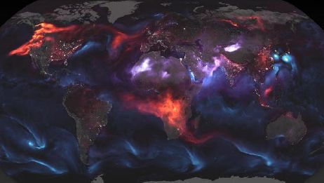
Figure 4.2. Emissions of substances into the Earth’s atmosphere (source: © NASA/J. Stevens and A. Voiland). For a color version of this figure, see www.iste.co.uk/sigrist/simulation2.zip
COMMENT ON FIGURE 4.2.– This image, produced on Thursday, August 23, 2018 by the NASA Earth Observatory, shows the emissions of different components into the atmosphere: carbon dioxide in red (resulting from human activities, or natural hazards, such a huge fires – as occurred, for instance, in 2018 in the United States or in 2019 in Brazil), sand in purple and salt in blue.
Aerosols are suspended particles, emitted, for example, during natural phenomena, such as volcanic eruptions or storms (in Figure 4.2, salt and sand, for example), or by human activities. They tend to cool the atmosphere by contributing to the diffusion of solar energy: for example, a decrease in global temperatures was observed after the eruption of Mount Pinatubo in 1991. For 2-3 years, it interrupted the global warming trend observed since the 1970s [SOD 02].
Some gases in the atmosphere (water in the form of vapor in the clouds, CO2 or other chemical compounds such as methane or ozone) tend to warm the atmosphere. Absorbing light in the infrared range, they block the re-emission into space of the thermal energy received on the ground under the effect of solar radiation. Without this greenhouse effect, our planet would simply be unbearable, with an average temperature of around –18°C [QIA 98].
While the effect of aerosols tends to disappear quickly (within a few months or years) when they fall to the ground, the influence of greenhouse gases is much longer. It is also delayed from their release, as they persist longer in the atmosphere (a few years or decades) and accumulate there – thus gas emissions, and especially CO2 emissions, receive special attention. The latter are the result of both natural cycles (e.g. plant and tree growth) and human activities, and it is a well-known fact that releases from various sources have steadily increased over the past two centuries (Figure 4.3).
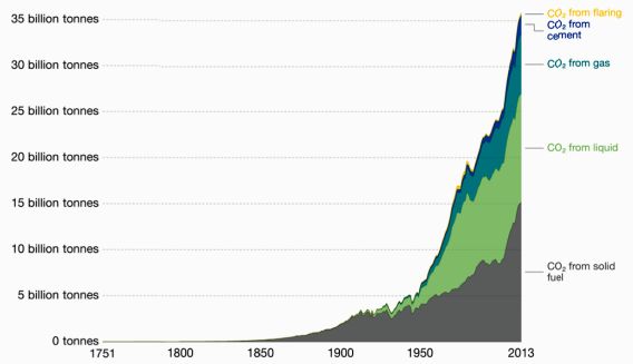
Figure 4.3. CO2 emissions from different sources (source: Our World in Data/https://ourworldindata.org/co2-and-other-greenhouse-gas-emissions). For a color version of this figure, see www.iste.co.uk/sigrist/simulation2.zip
Thus, in 2017, the concentration of CO2 in the atmosphere near the Earth reached a record value of 405 ppm, the highest in recent atmospheric history. The values estimated using polar or mountain ice surveys can go back nearly 800,000 years: they also indicate that the 2017 level is unprecedented over this period [BLU 18].
Changes in temperatures on Earth mainly depend on these effects of absorption or reflection of solar energy (influenced by aerosols and greenhouse gases), terrestrial thermal emissions, and exchanges between the oceans and the atmosphere. The most recent data show that the average temperature on Earth has been steadily increasing since the 1960s (Figure 4.4).
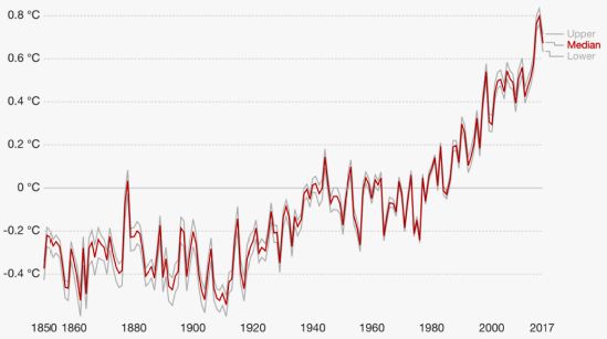
Figure 4.4. Evolution of the average temperature at the Earth’s surface from 1850 to 2017 (source: Our World in Data/https://ourworldindata.org/co2-and-other-greenhouse-gas-emissions). For a color version of this figure, see www.iste.co.uk/sigrist/simulation2.zip.
COMMENT ON FIGURE 4.4.– The figure represents the evolution of the average global temperature, in terms of deviation from a reference (here, the average temperature observed over the late 19th Century). The data presented are the result of statistical processing: the red curve represents the median value of the data (the temperatures are divided into two sets of equal importance) and the gray curves the temperatures below 5% of the minimum values and above 5% of the maximum values (extreme values are thus eliminated). The average value, obtained from temperatures measured at different stations, by definition masks temperature disparities in different parts of the planet. “Global warming” refers to the steady rise of Earth’s average temperature.
To what extent do CO2 emissions, and more broadly all substances released by human activities, influence this climate change? Based on mathematical models and reflecting the current understanding of climate mechanisms, numerical simulation, developed and refined since the 1970s, is a tool that scientists use to answer this question.
4.2. Atmosphere and meteorology
The semifinal of the Rugby World Cup, October 13, 2007, Stade de France, pits the starting 15 English ‘Roses’ against 15 French ‘Blues’: the rivalry between the two nations is no longer historical or political, it is that particular day, sporting! For 80 minutes, the players ran after an oval shaped ball that was more capricious than usual. Carried by strong winds, it condemned them to a game entrenched in the mud. Wet by frivolous rain, the passes appear blurry. Only one try is scored in the game, feverish and uncertain, while other points are obtained by penalties. With two minutes remaining, the whites camped in front of the blue poles despite the bad weather and Jonny Wilkinson – one of the most talented players of his generation – made a memorable coup de grâce to the French team, a drop perfectly adapted to the weather conditions.
For England’s number 10, it was not the first time he had tried it. In the final of the previous competition against Australia, he gave his team a world title with a kick in the last seconds of a match, at the end of which the outcome was just as uncertain. Jonny Wilkinson was personally interested in quantum mechanics, out of intellectual curiosity. For the French physicist Étienne Klein, with whom he exchanged at a conference organized at the École Nationale Supérieure de Techniques Avancées [WIL 11], this outstanding sportsman had, through his practice of rugby, intuitively understood certain concepts of quantum mechanics. Conquest by moving backwards, ball with random rebounds, part of the interpretation of the game phases by a referee-observer who influences the progress of the current experience: rugby is also a sport that defies classic mechanics.
If the weather conditions had been different on that unfortunate semifinal day for the French, would the match have been different?
4.2.1. Global and local model
Whether in sport, agriculture, fishing, industrial production, transport, tourism and leisure, our dailiy life is largely conditioned by the vagaries of the sky, clouds or winds. Knowing the weather in a few hours or days, with a sufficient level of reliability to avoid inconvenience, is an increasingly important issue for many economic sectors.
Wind speed, air temperature and pressure, atmospheric humidity are the quantities that weather forecasts seek to calculate at different scales. Météo-France contributes to the development of models that meet this objective.
A global model reports on changes in the atmosphere and is based on various assumptions. In particular, the Earth is supposed to be perfectly spherical, covered with a mantle of several atmospheric layers, with a significant thickness (up to 100 km above sea level, i.e. 25 times the altitude of Mont-Blanc!). The global model provides information on weather conditions over the entire surface of the planet: these are used to provide information for local models, for example, at the scale of a country. Cloud formation, air mass flow, sometimes spectacular as in a storm or typhoon: meteorological modeling uses fluid mechanics equations. The simulations obtained with the global model are based on a mesh of the atmosphere using elements or volumes whose size determines the accuracy of the calculation (Figure 4.5).
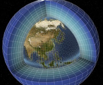
Figure 4.5. Meshing of the atmosphere (source: © ISPL/CEA-DSM). For a color version of this figure, see www.iste.co.uk/sigrist/simulation2.zip
For the global model, the elements have a dimension of just under 50 km on each side, for the local model, about 1–10 km. The Earth’s surface area is about 515 million km2: it is therefore covered by 5 million elements within 100 km2. For local models, the volumes are about 1 km apart. The surface area of France is 550,000 km2: as many elements of 1 km2 are used for the simulations, 100 times more to take into account the variation of physical quantities with altitude.
A meteorological simulation thus calls for between 5 and 500 million elements (by comparison, an industrial simulation of a ship or aircraft may require a few million elements). On each element, there are many quantities to calculate: temperature, pressure, humidity and velocity in three directions. Nearly, 1 billion pieces of data to calculate at different times during the simulation.
An additional difficulty arises for simulations: the equations of fluid mechanics represent different phenomena, such as the advection and propagation of physical quantities, whose evolution over time takes place at very different paces. In order to correctly represent these phenomena, it is necessary to use a time step that is smaller the higher the spatial resolution. This ensures the stability of the calculation. When the forecasts extend over a 10-day period, simulation times would become prohibitive. The calculations then use appropriate algorithmic techniques, allowing these phenomena with contrasting dynamics to be simulated separately.
Country-scale simulations (Figure 4.6) find data from the global model useful, for example, to determine boundary conditions (i.e. the meteorological conditions at the edges of a region) and also useful for local models. In particular, they describe the evolution of areas of high or low pressure and all relevant information for weather reports: presence and composition of clouds, storms, rain, snow and fog.
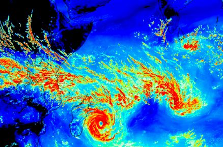
Figure 4.6. Numerical simulation of a cyclone off the island of Madagascar (source: ©CERFACS). For a color version of this figure, see www.iste.co.uk/sigrist/simulation2.zip
Each simulation needs data on which to base its calculations. The initial conditions give the most accurate possible representation of the state of the atmosphere at the beginning of the simulation. Data assimilation makes it possible to determine them.
Conventional meteorological data comes from the historical network of ground stations or observation satellites – the latter nowadays providing the bulk of the information needed for forecasting. They are supplemented by opportunity data obtained from shipping and airline companies. Winds, clouds, humidity, temperature and air pressure also influence the transmission of information on various systems, such as GPS. By observing the effects using models, it is possible to trace their cause – such as defining a guitar geometry based on the expected sound qualities: scientists also speak of “inverse methods”. These indirect data have complemented conventional data for the past 20 years or so.
The quantities measured directly or estimated indirectly represent 5–10 million data: a significant quantity and yet insufficient to be used by simulations, which require nearly 1 billion! In order to complete the missing information, data assimilation uses the results of previous numerical simulations. This combination of collected and calculated data makes the particularity of a calculation method and code developed by Météo-France, in partnership with the European Centre for Medium-Range Forecasts.
Data assimilation is an optimization problem: the state of the atmosphere is represented by a vector, a collection of calculated physical quantities, making the assimilation error as low as possible. In mathematical terms, such a problem is written as ![]() represents the set of possible values for the quantities x. φ measures the sum of the difference between the state being searched and the observations, on the one hand, and the difference between the same state and the previous numerical simulation, on the other hand. The difficulty is to find a minimum value for a function that depends on 1 billion variables! In order to find the such value, mathematicians use methods similar to those experienced in the sensitive world. Like a skier who runs down a slope looking for the most optimal path in terms of movement and disruption, thus adapting to the terrain, a descent algorithm rolls toward the lowest point of an uneven surface (Figure 4.6 in the first volume). In a few iterations, it makes it possible to find a minimum value for a mathematical function – sometimes depending on a very large number of variables.
represents the set of possible values for the quantities x. φ measures the sum of the difference between the state being searched and the observations, on the one hand, and the difference between the same state and the previous numerical simulation, on the other hand. The difficulty is to find a minimum value for a function that depends on 1 billion variables! In order to find the such value, mathematicians use methods similar to those experienced in the sensitive world. Like a skier who runs down a slope looking for the most optimal path in terms of movement and disruption, thus adapting to the terrain, a descent algorithm rolls toward the lowest point of an uneven surface (Figure 4.6 in the first volume). In a few iterations, it makes it possible to find a minimum value for a mathematical function – sometimes depending on a very large number of variables.
In addition, data assimilation techniques, coupled with the computational power applied to simulations, make it possible to perform emergency calculations, for example to predict intense and sporadic climatic phenomena, such as heavy rainfall.
Using simulation and data assimilation, Météo-France carries out four daily forecast cycles for the global model, at 12:00 pm, 6:00 am, 12:00 am and 6:00 pm. For 4-day forecasts, which we have access to, for example, with an Internet application, calculations take 1 hour 30 minutes to assimilate data and 30 minutes to perform a simulation. An achievement performed every 6 hours!
In recent years, these forecasts have been accompanied by a confidence index. The latter is a sign of an evolution in methods, made possible by increasingly computing capacities and by an evolution in computing methods. They now integrate uncertainties in the input data and assess their influence on the outcome of the forecast. This more probabilistic conception of simulation is one of the avenues for innovation in numerical methods in meteorology – as in other fields.
The methods will have to evolve further, for example, by integrating the advances of Big Data [BOU 17]. Simulations and observations, but also traces of each other’s digital activities with the connected objects: stored, collected and processed by Météo-France, data related to weather and climate await the next algorithmic innovations to deliver their information and contribute to the development of new prediction methods, such as real-time information or warning devices, etc.
4.2.2. Scale descent
The Route du Rhum is one of the prestigious solo sailing races and its progress is fascinating beyond the circle of regatta lovers. In 1978, its first edition was won by Canadian skipper Mike Birch. Departing from Saint-Malo in France, he reached the finish line in Guadeloupe after 23 days, 6 hours, 59 minutes and 35 seconds of racing, only 98 seconds ahead of his pursuer, the French skipper Michel Malinovski (1942–2010). Forty years later, the same scenario seems to be emerging: for the 2018 edition, the Frenchmen François Gabart and Francis Joyon are in the lead off Guadeloupe. At this stage of the race, weather data are crucial for sailors.
On November 11, 2018, French meteorologist Yann Amice, founder of Metigate, simulated wind conditions around the island (Figure 4.7). For sailing specialists, the calculation suggests that the finish of the race presents many difficulties for skippers
- – will the finish be as competitive as in 1978? The 2018 race turned out to be different, perfectly illustrating the aphorism attributed to Niels Bohr in the first volume… Let us take a look at the simulation of wind conditions in 2018. It is carried out on a square area of 180 km, composed of calculation cells with 3 km on each side
- – a resolution which is essential in order to generate useful data for navigators.

Figure 4.7. Simulation of wind conditions around: the wind scale is indicated in knots (source: www.metigate.com) For a color version of this figure, see www.iste.co.uk/sigrist/simulation2.zip
Blandine L’Heveder, an expert in weather and climate simulation, contributed to the calculations:
“These simulations are based on ‘high-resolution’ meteorological techniques: the aim is to produce realistic data in given geographical areas with high accuracy. Typically, calculations are performed with a resolution of about 1 kilometer – and in some cases, it may be less! The calculations are based on ‘downscaling’ techniques: starting from meteorological data at a resolution of 25 kilometers, we simulate successively the meteorological conditions on domains whose resolution decreases: 15 kilometers, 3 kilometers… then 1 kilometer. At each step of the calculation, we use the results obtained at the upper scale to set up the initial and boundary conditions of the calculation of the current scale.”
This scale descent is carried out in steps of resolution (Figure 4.8), the calculation taking place in an immutable sequence.

Figure 4.8. Downscaling principle: local simulation on the Marseille region based on global data on the South-East of France (source: www.metigate.com). For a color version of this figure, see www.iste.co.uk/sigrist/simulation2.zip
COMMENT ON FIGURE 4.8.– The figure schematically represents the principle of a downscaling: from a global meteorological simulation result, for example with a resolution of 25 km, it is possible to obtain simulations at finer scales, for example with a resolution of 3 km.
“The first part of the calculation is that of fluid dynamics: it involves solving the flow equations (Navier–Stokes equations) on a 3D mesh and calculating the pressure, velocity and temperature fields. Indeed, the expression of horizontal and vertical variations of the various quantities, as well as that of the transport of these quantities by the wind, involve values in the neighboring meshes. The second part of the calculation is that of the physics of the atmosphere. Radiative phenomena (radiation, absorption, diffusion by clouds and gases in the atmosphere), and so-called ‘sub-grid’ effects (evolution of turbulence, formation of water drops, interactions related to friction with the ground induced by the presence of vegetation, construction, etc.) are represented. These phenomena depend on different factors that the models translate into equations called ‘parameterizations’. This calculation step takes place along the meshes of a vertical column and is regularly inserted between the fluid dynamics calculation steps. Carried out on average once after five dynamic steps, this process makes it possible to describe, for example, the rainfall or the turbulent transport of water vapor evaporating on the ocean surface. Similarly, the ground effect, which may be characterized in particular by friction, influences the flow profile up to an altitude of nearly 1,000 meters! It is essential to represent it and to do so, we use data from field surveys.”
Different models operate during this last stage and all the “art of prediction” of the experts is mobilized in order to achieve the most accurate modeling possible. A constraint: that of calculation times!
“Calculation techniques are limited by an essential constraint: the step of temporal resolution is imposed by spatial resolution. In particular, a numerical condition requires that the calculated information must not propagate at a speed greater than that of a space mesh over a calculation time step – otherwise, the simulation loses all meaning, indicating a mathematical result (the latter is known as the ‘Courant-Friedrich-Lewy condition’, after the mathematicians who helped to understand and formalize it). Thus calculations with low spatial resolution take the longest time and may only be accessible with supercomputers. Simulating 48 hours of weather over a 60-kilometers-side region with a 1 kilometer resolution requires only 30 minutes, using 32 computing cores! According to the same principle, it is possible to descend to smaller scales: up to 50 meters, 10 meters, etc., using other types of models.”
The weather tomorrow or in 10 years’ time is gradually becoming less elusive, but the result of the next Rugby World Cup or the ranking of the next sailing race remain uncertain until the final whistle blows or the arrival at the port!
4.3. Oceans and climate
After the Second World War, a world dominated by the United States and the Soviet Union emerged. In April 1961, the first man who reached in space was Russian. In July 1969, the first men to tread the lunar ground were American. A Cold War legacy may be embodied in the race between the two powers to space. Communications, transport, meteorology, and observation of the Earth: nowadays, a large part of humanity benefits directly from this conquest. International space missions have made it popular, thanks in part to outstanding personalities, including those mentioned at the beginning of this chapter, or more recently the likes of French astronaut Thomas Pesquet [MON 17, PES 17].
The Silent World, the realm of the deep ocean, can arouse the same enthusiasm as the conquest of space, with the oceans being, for some, the future of humanity. In 1989, Canadian filmmaker James Cameron, passionate about the seas and oceans and director of Titanic [CAM 97], staged the beauty and mystery of the deeps in a science fiction film, symmetrical of those dealing with space exploration in search of otherness. The Abyss is an adventure immersed in the infinite depths of the oceans and the human soul [CAM 89], perhaps illustrating these verses by French poet Charles Baudelaire (1821–1867): “The sea is your mirror; you contemplate your soul in the infinite unfolding of its blade – and your mind is no less bitter abyss!” (L’Homme et la Mer [BAU 57]).
The oceans cover nearly 70% of the world’s surface and are the largest water reserve on our planet, accounting for 95% of the available volume. They also host the majority of living species on Earth [COS 15] – drawing up an inventory of them is a fundamental challenge for biodiversity knowledge: more than 90% of marine species are not yet fully described by scientists [MOR 11]. Contributing to the production of most of the oxygen we breathe, and accumulating carbon dioxide at the cost of acidifying their waters, the oceans generate many ecosystem services that allow humanity to live on the blue planet.
Ocean modeling is a key tool for scientists to understand some of the mechanisms that are critical to the functioning of ocean ecosystems, the future of marine biodiversity and climate change.
4.3.1. Marine currents
Their tremendous capacity to absorb CO2 or thermal energy makes the oceans the main regulator of climate. By mixing huge quantities of water, marine currents help to circulate the heat of our planet (Figure 4.9): a global flow whose mechanisms have been known for nearly a century, and whose importance on climate is nowadays the subject of many scientific studies.

Figure 4.9. The main currents of the North Atlantic (source: © IFREMER). For a color version of this figure, see www.iste.co.uk/sigrist/simulation2.zip
COMMENT ON FIGURE 4.9.– The map shows the main currents of the North Atlantic Ocean. Warm currents (red and orange) flow on the surface, moving up from southern areas to northern areas, whereas cold currents (blue) move deep in the opposite direction. Very cold and low-salt currents are measured in the boreal zones off Greenland and Canada (green on the map). While the North Atlantic is the largest engine of the “ocean conveyor belt”, other loops exist in other regions, such as the Pacific or the Indian. Carried away in these currents, a particle of water travels around the planet in a thousand years! The measurement campaigns at sea make it possible to understand the currents. France and the United Kingdom, with their partners, organize expeditions represented on the map by the black lines: between Portugal and Greenland (black spots) and between West Africa and Florida (black crosses).
Different models make it possible to understand ocean dynamics, as Pascale Lherminier, researcher at IFREMER*, explains:
“As close as possible to physics, ‘primitive’ equations (such as the Navier-Stokes equations) describe the dynamics of fluids and ocean currents. A simulation based on these equations is theoretically possible, but requires a very significant modeling and computational effort. ‘Theoretical’ equations may be deduced from the complete physical models: separating different effects, they constitute an ideal ocean model that makes it possible to understand each of them. ‘Large-scale’ equations reduce the size of models by filtering some of the information and physical phenomena. They allow simulations with a good compromise between computational cost and physical accuracy. This ‘equation-based’ modeling nowadays coexists with ‘data-based’ modeling. Data assimilation techniques allow, for example, to determine the conditions of a calculation by a means of a mathematical expression, while learning techniques make it possible to represent a physical process in the form of a ‘black box’, built from statistical observations.”
These different models are used in ocean science, as in the other fields we cover in this book. The dynamics of the oceans remain very complex and data are still scarce, as scientists do not have as much information as for the atmosphere, for example. While satellites provide surface data, other systems (probes, floats) provide depth measurements (Figures 4.10 and 4.11).

Figure 4.10. Offshore measurement system
(source: © P. Lherminier/IFREMER)
“‘Argo’ is a program initiated in the 1990s to provide the international scientific community with ocean data. Nearly 4,000 floats are deployed in the oceans. Deriving freely, they collect information at depth, up to 2,000 or 4,000 meters today – the main part of the heat transfer phenomena occurring at a depth of about 2,000 meters. In addition, many countries are organizing measurement campaigns at sea, coordinated by an international program (Go-SHIP) to ensure better complementarity. With the OVIDE program, we carry out measurements every two years of different physical quantities characterizing the ocean: velocity, temperature, salinity, pressure, dissolved O2 and CO2, acidity, etc. Between the coasts of Portugal and Greenland, the ship carries out about 100 measurement profiles, from surface to bottom, at points about 40 kilometers apart.”
The information collected is particularly useful for “reverse modeling”, which combines data to calculate physical quantities representing the state of the ocean from measurements [DAN 16, MER 15]. The transition from the second to the first is accomplished by means of “simplified equations”, which are established from the “primitive equations”. Inverse models allow to reconstruct an image of mass and heat transport on a depth profile, overcoming many technical difficulties:
“On a hydrodynamic section, i.e. on a surface-to-bottom line, we calculate the current by vertical integration of the pressure anomalies. Filtering transient processes at small scales of time and space, the ‘integrated’ data is more reliable than the ‘averaged’ data, which can be parasitized by small fluctuations. One of the difficulties is that the integration process does not define a value in a unique way: additional information is needed. For example, it is possible to assume that the deep current is zero, but this assumption is not verified in practice. Missing information is obtained, for example, by measuring ocean elevation: surface data, provided by satellite observations, can be used to complete the current profile…”
As some of the latest simulation results available show the variability of ocean currents (Figure 4.12), it is now up to scientists to interpret these results:
“Ocean transport varies greatly from year to year and its 10-year variations are even greater! It remains to be understood whether this phenomenon is due to current climate changes or whether its causes are of a different nature. The existence of these cycles is not yet well fully explained…”
While scientists, just like James Cameron’s film, find that the deep ocean retains many enigmas, the depths of their science are constantly filling up – and knowledge of marine currents is spreading in many areas (Box 4.1).
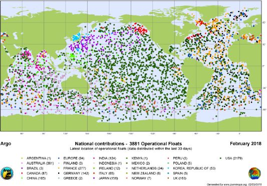
Figure 4.11. The international program “Argo” collects oceanological data through a network of nearly 4,000 floats spread throughout the world’s seas and oceans (source: www.commons.wikimedia.org). For a color version of this figure, see www.iste.co.uk/sigrist/simulation2.zip
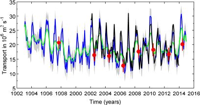
Figure 4.12. Evolution of ocean transport relative to the North Atlantic “conveyor belt” between 1992 and 2016 (source: © IFREMER/CNRS/UBO). For a color version of this figure, see www.iste.co.uk/sigrist/simulation2.zip
COMMENT ON FIGURE 4.12.– The figure shows the variations between 1992 and 2016 in volume flow in the North Atlantic from the tropics to the northern seas at the surface, and in the opposite direction at depth. Built from models fed by measurements at sea, the data show annual cycles, with flows varying between 10 and 30 million m3 per second, and 10-year cycles, with flows varying between 15 and 25 million m3 per second.
4.3.2. Climate
What about the climate? In contrast with the weather forecast, which is concerned with changes in the “very short-term” (hours or days) of the atmosphere and oceans in various location, climate study focus on long-term variations (occurring in decades, centuries or even millions of years). Understanding and predicting the likely evolution of Earth climate is a current scientific challenge to which modeling contributes.
Variations in the states of the atmosphere and oceans are the result of a large number of phenomena that can be represented numerically. A climate model may therefore be based on the coupling between the dynamics of the atmosphere, with the models mentioned above, and that of the oceans. The equations of fluid mechanics are present behind the simulations. They are complemented by various other factors, which describe the variety of interactions in the climate system:
- – interactions between chemical species in the atmosphere (some resulting from human or plant activities, such as carbon dioxide, methane or ozone emissions) and energy transfers by radiation, emitted or absorbed as a result of the presence of these chemical species;
- – interactions between the continental biosphere (photosynthesis, respiration, plant evapo-transpiration) and the atmosphere;
- – interactions between ocean bio-geochemistry (plankton, carbon compounds, etc.), the carbon cycle in the global climate system and ocean circulation;
- – interactions between sea ice (model of the same type as the ocean or atmosphere model), the ocean and the atmosphere, or between continental ice, land and the atmosphere.
In addition, “radiation forcing” describes the amount of energy received by the Earth’s atmosphere from solar radiation and is a key element in climate simulations, whose ability to account for such complex interactions improved over decades. The models used today for climate studies compiled and assessed by the Intergovernmental Panel on Climate Change (IPCC)3 integrate all possible phenomena (Figure 4.18).
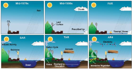
Figure 4.18. The complexity of climate prediction models has increased in recent decades [TRE 07]
COMMENT ON FIGURE 4.18.– The figure shows the evolution of modeling assumptions in climate studies from the 1970s to the present. Relatively simple in origin, the models take into account solar radiation, precipitation and CO2 emissions into the atmosphere. Climate models are becoming richer and gradually integrating other effects. First, the influence of clouds in the atmosphere and glaciers in the oceans, then all known phenomena: volcanic activity, the complete carbon and water cycle, emissions of other gaseous substances and aerosols, as well as the chemical reactions they undergo in the atmosphere. FAR, SAR, TAR and AR4 refer to the first four reports published in 1990, 1995, 2001 and 2007. The fifth report was released in 2014, and the latest report was published in 2018 (source: https://www.ipcc.ch/publications_and_data/publications_and_data_reports.shtml)
Ocean modeling represents the dynamics of marine currents, rendered by fluid mechanics equations. This is influenced by salinity effects, ice or marine vegetation in some ocean regions. Atmosphere and oceans evolve simultaneously. Wind and heat exchange influence the sea surface state, while ocean temperature is transmitted to the atmosphere. Simulations account for these mechanisms by coupling calculation tools specific to the digital representation of the atmosphere and the ocean.
Before each calculation, the initial state of the oceans is determined by data assimilation methods. The data for wave height, temperature, salinity, etc. come from observations and measurements at sea. They make it possible to force the physical model to take as the initial condition of the calculation the state closest to that observed, in order to give the greatest possible accuracy to the simulations. The equations will then do the rest to represent the evolutions of the ocean.
The resolution of the simulations has constantly been refined (Figure 4.19). In particular, some calculations use the most efficient computational means at disposal – such as high performance computing (Chapter 3 of the first volume) – making it possible to study many scenarios. Gérald Desroziers, research engineer at Météo-France, explains:
“A simulation is nowadays typically based on 10 million calculation points, arranged with a resolution of 50 to 100 kilometers. This resolution is imperative when it comes to representing the atmosphere and oceans globally! One month of computation time makes it possible to produce data from about 10 scenarios of evolution over 100 years: these computation times are perfectly acceptable for research studies.”
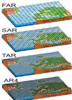
Figure 4.19. The geographical resolution of successive generations of climate models has steadily increased [TRE 07]
COMMENT ON FIGURE 4.19.– The figure represents the successive generations of models used by scientists studying climate change by the means of simulations: it shows how their resolution has increased, taking the example of Northern Europe. The mesh size has typically increased from 500 to 110 km between 1990 and 2007. The latest generation of numerical models have the highest resolution and they are adopted for simulations of short-term climate change, i.e. over several decades. For long-term evolutions, simulations are conducted using the model of the previous generation in order to reduce calculation times. Vertical resolution is not represented, but has evolved in the same proportions as horizontal resolution: studies reported the first IPCC report used one ocean layer and 10 atmospheric layers to reach 30 atmospheric and oceanic layers in the latest generation of models. FAR, SA, TAR and AR4 refer to the four successive climate reports published by the IPCC in 1990, 10997, 2001 and 2007, respectively.
With different scenarios, on average between 50 and 100 are needed, scientists have access to statistical data to study the influence of different model parameters (e.g. moisture content and concentration of a chemical species) on possible climate states. As with weather forecasting, this approach makes it possible to accompany the calculations with a reliability estimate, which is essential to propose scenarios that may realistically contribute to anticipating climate change.
Simulations can be used, for example, to model a probabilistic ocean. Based on different hypotheses, they provide access to mean ocean states and estimate the variability of the physical quantities that characterize them. Calculations allow the reproduction of the past evolution are of state of the oceans and can represent its variability over time (Figure 4.20).

Figure 4.20. Calculation of ocean surface temperature. For a color version of this figure, see www.iste.co.uk/sigrist/simulation2.zip
COMMENT ON FIGURE 4.20.– The figures represent the numerical simulation results of the ocean surface temperature. Calculations are made using the OCCIPUT (Computing platform for volumetric imaging) code, developed at CERFACS (European Center for Research and Advanced Training in Scientific Computing). The first figure represents the surface temperature of the oceans in degree Celsius on October 1, 1987. The daily average temperature obtained by simulation is between 0°C (black and blue areas) and 30°C (red and white areas). The second figure represents the intrinsic variability of this temperature on December 31, 2012. This is a 5-day average calculated using 50 simulations over 45 years of observation. The variability is between 0–0.2°C (in black and blue) and 0.8–1°C (in red and white) [BES 17, LER 18, SER 17a].
In France, CERFACS* works in collaboration with Météo-France to conduct climate simulations that contribute to IPCC reports. The data from the simulations are compared with measurements and attest to the validity of the models. Their reliability to predict possible ocean and climate changes is established (Figure 4.21), as Olivier Thual, a researcher at CERFACS, explains:
“Models are nowadays able to accurately represent past climate changes. They help to predict its variability in a way that is quite convincing to the scientific community. Simulation has become a major tool of interest in climate change studies.”
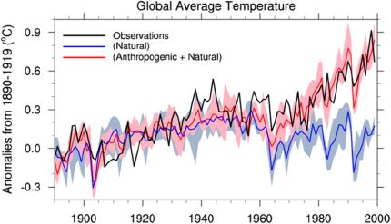
Figure 4.21. Contributing to the study of climate, numerical modeling is used to understand the influence of human activities on the global temperature evolution observed in the 20th Century [MEE 04] For a color version of this figure, see www.iste.co.uk/sigrist/simulation2.zip
COMMENT ON FIGURE 4.21.– A set of numerical simulations conducted in 2003 using global models allows to study the influence of various known factors on climate change. Two of them are of natural origin (solar radiation and volcanic emissions), the others correspond to certain human activities (including emissions of various aerosols and greenhouse gases). The simulations are compared with available temperature data: the calculations highlight the influence of factors attributable to human activities – and explain the temperature increase observed since the 1960s. Modeling, whose finesse has increased since 2003 (Figures 4.16 and 4.17), contributes to the development of the various climate change scenarios, as presented in IPCC reports. The figure shows the evolution of the difference between the mean global temperature and its observed value over the period 1890–1919. This evolution is measured and simulated over the period 1890–2000. The global average value is an indicator that does not reflect local variations. However, similar trends have also been confirmed for temperature evolutions in various regions of the world. These conclusions have been challenged by some scientists, who think that models fail to fully understand or explain meteorological phenomena and cannot reliably justify them [LER 05]. Science in general is an ongoing process that proceeds through discussion and interpretation of scientific results to reach consensus. To this day, the scientific community largely agrees on these conclusions elaborated with the knowledge available. Climate change continues to be positioned at the core of numerous researches, some using both observation data and simulation results, in order to further improve understanding and refine predictions.
Climate simulations are based on a wide variety of modeling: the results of about 30 climate models developed around the world are analyzed in IPCC reports, as Blandine L’Heveder explains:
“This diversity of models is essential for assessing the uncertainty associated with climate modeling. In a set of calculation results, the median value of the results divides them into two subset of equal weight. Scientists assert that the median of the data set produced by climate models is a relevant value: providing estimates close to the measurement data, it attests to the overall validity of historical climate simulations.”
It is partly thanks to scientific computation that the recommendations of the IPCC experts are constructed – and the different scenarios they produce give indications on the share of climate change may be influenced by human activity (Figure 4.23).
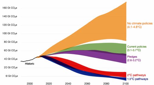
Figure 4.23. Possible evolution of the Earth’s temperature under different greenhouse gas emission assumptions
COMMENT ON FIGURE 4.23.– The figure shows different scenarios for the evolution of the global average temperature by 2100 under different greenhouse gas emission policies. Greenhouse gas emissions are measured in tons of CO2 equivalent. “No climate policies the scenario evaluates the evolution of emissions if no climate policy is implemented; it concludes that there is a probable increase in temperature between 4.1 and 4.8°C by 2100, taking as an initial situation the global temperatures observed before the industrial era. “Current climate policies”: the scenario forecasts a warming from 3.1 to 3.7°C by 2100, based on current global policies. “National pledges”: if all countries meet their greenhouse gas emission reduction targets as defined under the Paris Agreement, it is estimated that global warming will range from 2.6 to 3.2°C by 2100. The Paris Agreement, signed in 2016, sets a target of 2°C. “2°C Pathways” and “1.5° pathways”: these two scenarios show the effort required to limit warming to 2°C and 1.5°C, limits considered acceptable by many scientists in order to avoid significant changes on our living conditions on Earth. Scenarios for increasing global temperature below 2°C require rapid reductions in greenhouse gas emissions: in a context where energy is a major contributor to greenhouse gas emissions, the task for humanity seems very ambitious (source: OurWorldinData/www.ourworldindata.org).
The consequences of climate change are potentially universal and widespread – economy, security, infrastructure, agriculture, health and energy [MOR 18]. Anticipating them and equipping humanity with the technical, legal and political means to adapt to them is undoubtedly one of the essential challenges we face at the beginning of the 21st Century. While, from China to the United States, via Europe, humanity once again imagines projecting itself into space in order to reach Mars or exploit the resources of the Moon [DEV 19, DUN 18, PRI 19], atmospheric and climate modeling, as well as the message from astronauts who have experimented with the Overview Effect (Figure 4.24), may remind everyone that our destiny is, at least in the short term, terrestrial – that is, essentially, oceanic.
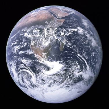
Figure 4.24. Blue Marble: Earth photographed from space during the Apollo 17 mission on December 7, 1972
(source: ©NASA)
- 1 Available at: https://earthobservatory.nasa.gov/images/86257/an-epic-new-view-of-earth. From these images, French engineers Jean-Pierre Goux [GOU 18] and Michael Boccara developed Blue Turn. An application that offers everyone a unique, intimate and interactive experience of the earth totally illuminated and rotating, seen from space. A numerical simulation of the visual experience reserved until now for astronauts only (available at: www.blueturn.earth).
- 2 Available at: http://plasticadrift.org/.
- 3 The IPCC is an intergovernmental body of the United Nations aimed at providing the world with a scientific view of climate change. It does not carry out original research (nor does it monitor climate or related phenomena itself), but it assesses published literature on the subject. IPCC reports cover the “scientific, technical and socio-economic information relevant to understanding the scientific basis of risk of human-induced climate change, its potential impacts and options for adaptation and mitigation” (see, for instance, https://www.ipcc.ch). IPCC reports may serve as ground for the elaboration of public policies – and, to some citizens, for individual action.