
5
Energies
Cinema was born at the end of the 19th Century; it was innovations in optics, mechanics and chemistry that made possible the development of photosensitive supports and mechanisms that, because of retinal persistence, synthesize movement. Some of the research preceding its invention had an essentially scientific purpose. At that time, the English photographer Eadweard James Muybridge, like the French native Etienne-Jules Marey, was interested in movement. Marey’s pictures show that during a gallop, for example, the horse does not have all four legs in the air! In 1878, Muybridge arranged a series of cameras along a racecourse. Triggered by the horse’s passage, the shots separated the movement (Figure 1.29 in the first volume) then allow an animated sequence to be obtained.
His experience preceded the invention of the American engineer Thomas Edison (1847–1931): in 1891, the kinetograph was the first camera to be used. In France, inventors Auguste and Louis Lumière (1862–1954 and 1864–1948) filed the cinematographer’s patent in 1895 – both a camera and an image projection camera, it was invented before them by Léon Bouly (1872–1932). The Lumière brothers shot a series of films with their camera and offered private screenings. The story of the first showing of the Arrivée d’un train à La Ciotat [LUM 85] recounts that the animated image of the train seeming to burst through the screen towards the audience sent them screaming and rushing to the back of the room.
5.1. The technical dream
The development of steam locomotives is also a symbol of the technical control of movement, made possible by thermodynamics and mechanics. In the early 19th Century, the United Kingdom saw the birth of these new machines and inaugurated the first railway line in 1812. The Middleton Railways received the Salamanca (Figure 5.1), built by British engineers Matthew Murray (1765–1826) and John Blenkinsop (1783–1831), it was the first commercially operated steam locomotive.
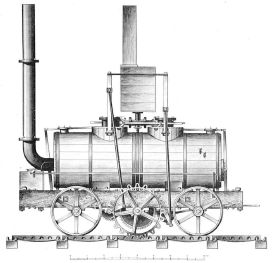
Figure 5.1. The Salamanca (1812) – schema first published in The Mechanic’s Magazine in 1829
(source: www.commons.wikimedia.org)
COMMENT ON FIGURE 5.1.– Power refers to the ability of a device or system (mechanical, chemical, biological, etc.) to deliver a given amount of energy in a given time. Before the advent of steam engines, humans often drew the energy necessary for hitch traction from horses. The English physicist James Watt (1736–1819) proposed horsepower as a unit of power measurement. Watt uses as a reference the power required to pull 180 pounds (or 0.4536 kg) of weight at a speed of 3.0555 feet per second (or 0.93 m/s) to overcome gravity (9.81 m/s2). The corresponding power is the product of this mass, speed and acceleration, approximately 745 W (the power unit being named in his honor). The French physicist and engineer Nicolas-Léonard Sadi Carnot (1796–1832) contributed to the development of thermodynamics, the science of heat. In 1824, he published a book acknowledged as being a major contribution to physics: Réflexions sur la puissance motrice du feu et sur les machines propres à développer cette puissance. Thermodynamics gave the framework for studying the functioning of thermal machines and designing them.
The Industrial Revolution marked the advent of machines and the growing importance they occupy in human life. They even became protagonists in their fiction, like The General, led by Johnnie, the character incarnated by American actor Buster Keaton (1895–1966) in his 1926 film. The machine is his second love, and when Annabelle Lee, his fiancée, is kidnapped by a squadron of the northern armies, it is with the help of the locomotive that he starts a steam chase race to save her [KEA 26]!
Large-scale access to mechanical energy has given humanity a new power to control and shape the world by pushing the limits of its physical constraints. French engineer Jean-Marc Jancovivi summarizes the history of the industrial revolution as follows:
“[It] is the invention of (machines) powered by a super-powerful energy that the human body does not know how to exploit directly […] It has allowed us to overturn in two centuries the multi-millenary hierarchy between environmental constraints and our desires […] We have set the borders of the world on our desires: it is the technical dream…” [JAN 18].
Realizing this dream, still restricted nowadays to the richest humans, requires a large amount of energy, the constant increase in which raises the question of the possible exhaustion of available resources for humanity (Figure 5.2). This energy consumption also exploits carbonaceous sources, which are partly responsible, along with other human activities, for the emission of many compounds into the environment.

Figure 5.2. Evolution of world energy consumption between 1965 and 2016 (source: Our World in Data/ https://ourworldindata.org/energy-production-and-changing-energy-sources) For a color version of this figure, see www.iste.co.uk/sigrist/simulation2.zip.
COMMENT ON FIGURE 5.2.– In 1965, world energy consumption was just over 40,000 TWh, and it was just over 145,000 TWh in 2016. In the same year, it breaks down by origin as follows: 40,000 TWh for coal, 50,000 TWh for oil, 40,000 TWh for gas; the 15,000 TWh are broken down into hydraulic (about 5,000 TWh) and nuclear (about 3,000 TWh) electricity and renewable energy sources (about 2,000 TWh). In 2016, more than 90% of the energy consumed by humans came from hydrocarbon combustion and 2% from renewable sources. 1 TWh refers to a thousand billion Watts per hour (unit of energy consumption). 1 TWh corresponds, for example, to the energy consumed by 10 billion people using a standard laptop computer for 2 h.
The energy sector, strategically contributing to the future of humans, makes extensive use of numerical simulation in order to:
- – optimize the operation of energy production machines;
- – demonstrate the expected safety and security requirements of sensitive installations;
- – research new energy production processes.
This chapter provides examples of these in different areas of the energy sector.
5.2. Combustion
In 1865, Jules Verne published From Earth to the Moon. The novel imagines the combination of different “technical bricks” (propulsion, aerodynamics, metallurgy, etc.) in order to realize the dream of conquering space [VER 65]. The writer also questions the motivations of humans and their relationship to technology. In this fictional world, it is partly the boredom, caused by the absence of conflict, which diverts the passion for the weapons of the Gun Club members toward the design of a super projectile, propelled to conquer the Moon. Verne thus anticipates more than half a century of history:
“They had no other ambition than to take possession of this piece of the continent from the air and to fly at its highest summit the starry flag of the United States of America” [VER 65].
Imagined by the French director Georges Méliès (1861–1938) [MEL 02] or the Belgian draftsman Georges Rémi (1907–1983) [HER 53, HER 54], the first steps of humans on the Moon became a reality when the American astronaut Neil Armstrong (1930–2012) took them on July 21, 1969, leaving his mark on the sea of tranquility [CHA 18].
The heroes of Verne and Méliès join the Selene star aboard a giant revolver ball pulled out of the earth’s gravity propelled by an immense cannon; in Hergé's comic strip, Tintin and his companions achieve their objective because of the atomic rocket imagined by Professor Tournesol. However, the 20th Century space conquest was achieved by means of combustion engines – propulsion based on the ejection of gas at high speed through a nozzle behind the launchers.
The take-off phase is one of the most critical: in order to optimize the design and improve the performance and robustness of launchers, engineers offer multiple technical solutions. Numerical simulation is a tool that helps nowadays to understand complex phenomena and guide design choices (Figure 5.3). Thierry Poinsot, a researcher in combustion simulation, points out that simulations of this type require significant resources:
“A simulation like that of the Ariane V rocket engine represents about 1,500 years on a computer equipped with a single processor! The use of supercomputers makes it possible to make these simulations accessible in only three weeks of calculation”.
Intensive exploitation of hydrocarbons (gas, oil and coal), pollution of urban areas, greenhouse gas emissions: combustion is a mechanical and chemical activity with multiple consequences on our environment. The most visible are water vapor or smoke emissions that modify landscapes and ecosystems. Behind the beauty of industrial flows observed at certain times of the day (Figure 5.4) are sometimes irreversible changes in the environment, to which our lifestyles contribute very significantly.

Figure 5.3. Back body calculation for Ariane V (source: ©ONERA). Fora color version of this figure, see www.iste.co.uk/sigrist/simulation2.zip
COMMENT ON FIGURE 5.3.– The calculation presented is based on the aerodynamic code “Elsa”, developed in France by ONERA. The flow of propulsion gases is turbulent and compressible, at Mach 0.8, so close to the speed of sound. This involves using calculation methods that account for both effects, which is a complex task. The proposed simulation, based on a modeling of the large scales of turbulence, requires nearly 120 million calculation points! It highlights the origin of the influence of the asymmetric fasteners of the boosters to the central body on the flow dynamics and lateral forces exerted on the launcher. A fine simulation requiring dedicated resources and skills, it produces valuable results for designers.
More generally, combustion indirectly affects the living conditions of billions of people in both industrialized countries and large emerging economies, which invest massively in this area. Today, 85% of the energy produced in the world comes from the combustion of hydrocarbons (Figure 5.2).
An observation made by the American photographer Alex MacLean, for example, with a series of photographs taken, among others, above industrial production sites, mining sites, etc. [MAC 08]. Combustion-engine-powered machines, and a large part of industrial activity, still contribute to meeting various human needs: food, heating, mobility. In a context where this trend has not yet been largely reversed in favor of alternative energy production methods, numerical simulation is being used to design more efficient and less polluting engines, as well as to test the efficiency of new resources, such as biofuels.

Figure 5.4. Smoke and steam rising above an industrial complex
(source: www.123rf.com/Shao-Chun Wang)
COMMENT ON FIGURE 5.4.– Thermodynamics, the science of heat, is based on two main principles. The first stipulates that the total energy of an isolated system is always conserved – and therefore remains constant (energy conservation principle). Energy cannot therefore be produced “ex nihilo” and can only be transmitted from one system to another: in other words, “one does not create energy, one transforms it”. The second establishes the “irreversibility” of physical phenomena, particularly during heat exchanges (thus thermal energy is spontaneously transferred from the hot body to the cold body). The second principle postulates the existence of a physical function, “entropy”, expressing the principle of energy degradation or characterizing the degree of disorganization, or unpredictability of the information content of a system. The second principle stipulates that the entropy variation of a system is always positive: energy “production” is therefore always accompanied by heat losses, waste production, etc. Thus, the second principle also serves to calculate the efficiency of a machine, an engine, a nuclear plant, a wind turbine, etc. It also indicates that there is no such thing as “renewable energy”, even if it is possible to produce energy from abundant sources (sun, wind, tides, etc.). Note that here we use, by extension of language, the term “energy production” to designate what physicians describe as “energy transformations”.
Combustion involves liquid or gaseous chemical compounds that flow and are burned in the thermal chambers of engines. The simulations are thus based on the equations of fluid mechanics, coupled with those of chemical reactions:
“Hundreds of different species and thousands of chemical reactions occur during combustion. This is the case, for example, for traditional fuels (kerosene, petrol) and bio-fuels, whose energy and chemical properties are to be assessed by calculation. The challenge of simulation is reporting on it. The latter has three major difficulties: the geometries studied are complex, the flows involved are highly turbulent and the kinetics of chemical reactions require highly accurate models”.
Chemical reactions occur in extremely short times, in the order of one nanosecond, or one billionth of a second (the equivalent of a day over a period of 1 million years). The simulation aims to represent them by calculating their evolution over time, the way they mix and are transported in the flow, which is also marked by turbulent phenomena, the latter thus being modeled as accurately as possible. For example, the ignition sequence of a gas turbine is a critical phase, usually not studied by engineers by means of a calculation, due to its complexity.
A full simulation was conducted by researchers in 2008 on one of the world’s leading supercomputers in the United States (Figure 5.5). It represents the actual geometry of the turbine, composed of 18 burners lit successively. It allows the study of the propagation of the ignition flame around the turbine perimeter. Turbulence is represented down to small vortex scales. The calculation requires tens of millions of CPU hours to simulate phenomena that actually occur in tens of milliseconds.
Optimizing the propulsive performance of an engine by limiting undesirable pollution effects requires a large number of simulations, the unit calculation cost of which is significant since the calculation models contain several hundred thousand unknowns.
Research and development in this field is a major strategic challenge: it involves many scientists in Europe, the United States and India or China, a country that invests heavily in the training of its engineers and equips itself with highperformance computing machines (Chpater 3 of the first volume). Maintaining the correct level of combustion calculation codes is, as with other tools, a major task.
The latter employs several dozen full-time engineers and researchers in the various R&D* centers interested in this theme. For them, it is a question of adapting the code to the thousands of processors of computing machines that are and will be used, for example, by manufacturers.
“Designing turbines only with simulation is however not an option these days: the stakes of reliability, robustness and propulsion performance are too high to do without one-scale prototypes. But simulation also complements the tests and thus helps to reduce design costs”.

Figure 5.5. Simulation of a gas turbine ignition sequence [BOI 08]. For a color version of this figure, see www.iste.co.uk/sigrist/simulation2.zip
COMMENT ON FIGURE 5.5.– The figure shows the gas state calculated in the body of a turbine 45 milliseconds after ignition. The initiation points of the sequence are indicated in red (top left and bottom right). The data shown are the gas velocities in the turbine axis (scale ranging from –20 m/s in light blue to +20 m/s in yellow), with the fastest gas temperatures superimposed (scale ranging from 273 K in turquoise to 2,400 K in red) and the flame front progression zone (bright light blue), corresponding to the maximum mass flow.
5.3. Nuclear energy
Some scientific discoveries are made by chance or by error, as is the case with radioactivity. In the late 19th Century, the German physicist Wilhelm Rögten (1845–1923) became passionate about cathode rays, generated by means of “Crooke tubes” – the ancestor of the tubes of the first television sets. With this device, he discovers a type of radiation capable of penetrating into matter (Figure 5.6): he designates these rays as the letter X, symbol of the unknown.

Figure 5.6. X-ray of the bones of a hand with a ring on one finger, Wilhelm Konrad von Röntgen, 1895
(source: Wellcome Collection/www.wellcomecollection.org)
COMMENT ON FIGURE 5.6.– On December 22, 1895, Wilhelm Röntgen made the first X-ray photograph in history by inserting his wife Anna Bertha’s hand between a Crookes tube and a photographic plate. He notes that “if you put your hand between the discharge device and [a] screen, you see the darker shadow of the bones of the hand in the slightly less dark silhouette of the hand”. The densest and thickest parts are the darkest on the plate: you can see a ring on the ring finger. Radiography was born! It is now widely used as an imaging medium in the medical field or in materials science – where it is part of non-destructive testing (Chapter 2).
5.3.1. Dual-use energy
The discovery of Rögten, presented in January 1896 at the Paris Academy of Sciences, intrigued the French physicist Henri Becquerel (1852–1908), who was, at the same time, interested in the phenomenon of fluorescence. In order to understand it, he worked with phosphorescent uranium salts deposited on photographic plates: exposed to the sun outdoors and later developed, they reveal the image of salt crystals. Becquerel attributed this phenomenon to Röntgen’s rays: he believed that solar energy is absorbed by uranium salt before being re-emitted in the form of X-rays, which then impresses the photographic plates. On February 27 the same year, while trying to expose his photographic plates, the weather was unfavorable to him: disappointed to see the sunlight stubbornly hidden behind the clouds, Becquerel put plates already impregnated with uranium salt in a cupboard, hoping for better conditions for a new experience. A few days later, on March 1, he still developed these plates and discovered that they were still impressed. The phenomenon was that of a spontaneous emission of radiation by uranium: Becquerel had just discovered radioactivity1.
French scientists Marie and Pierre Curie (1867–1934 and 1859–1906) followed Becquerel in their search for new “radioactive” substances, according to the terminology they had proposed. In 1898, they discovered Radium and Polonium. They suggested that radioactivity is an atomic phenomenon. “Something is happening inside the atom”: their insight disrupted the atomic theory inherited from Greek antiquity, according to which the atom is thought of as unbreakable.
In 1934, the French physicists Irene Curie (1897–1956) and Frederic Julliot (1900–1958) paved the way for artificial radioactivity by synthesizing a radioactive isotope of Phosphorus that does not exist in nature. Following Irene Curie’s work, German chemists Otto Hahn (1879–1968) and Fritz Strassman (1902–1980) discovered in 1938 that uranium bombarded by neutrons gave rise to two lighter elements. Nuclear fission is thus understood on the eve of the Second World War. In the context of this conflict, this discovery led to the development of weapons with unparalleled destructive power (Chpater 3 of the first volume). After 1945, nuclear energy was used in power plants: the first nuclear power plant was built in the United States in 1951, soon joined in the development of this technology by the Soviet Union (1954), Great Britain and France (1956) – these countries also acquiring nuclear weapons.
After experiencing significant development between the 1960s and 1980s, the nuclear industry, one of the most regulated, also became one of the most controversial. The shock caused by the disasters of Chernobyl in 1986 and Fukushima in 2011, and the management of hazardous waste it generates, has led the citizens of some Western countries to want nuclear energy to be phased out.
In 2015, the International Atomic Energy Agency (IAEA), the international observer body on nuclear energy and its civil or military applications, records 435 nuclear reactors in service worldwide. The majority are based on PWR (pressurized water reactors) and are located in the United States, France and Russia (after the Japanese reactors were shut down). The IAEA also estimates that by 2050, nuclear power will account for 17% of global electricity production. This increase will be particularly relevant in developing countries, according to the IAEA: 68 reactors are under construction in 15 countries, including 25 in China [SFE 16]. As an energy source claimed to be low in CO2 emissions2, nuclear power is, for some, one of the answers to the challenges related to energy production in the 21st Century.
The future of nuclear energy may be that of fusion, which experimental reactors nowadays aim to control. Whether based on one or the other of these techniques (Figure 5.7), nuclear energy control is partly based on numerical simulation, of which we will give some examples of its use.

Figure 5.7. Nuclear energy is obtained by fission or fusion: if the former is a proven technique, the latter remains to be invented
(source: www.shutterstock.com)
It should be noted that in France, there are many simulation tools whose development has been driven by the needs of the nuclear industry. Based on knowledge and innovations, largely funded by the community, not all of these tools have been commercially oriented and remain accessible to a broad global scientific community today.
5.3.2. At the heart of nuclear fission
A nuclear power plant produces electricity from the heat released by the decay of a heavy atom (formed by a large number of nucleons, such as uranium, plutonium, etc.), under the action of a neutron (Figure 5.8).

Figure 5.8. Nuclear fission (source: www.shutterstock.com). For a color version of this figure, see www.iste.co.uk/sigrist/simulation2.zip
COMMENT ON FIGURE 5.8.– Uranium is an element composed of heavy atoms. These atoms have a nucleus that can break into two smaller nuclei under the impact of a neutron. Since the neutron has no electrical charge, it can easily approach the nucleus and penetrate inside without being pushed back. Fission is accompanied by a large release of energy and, at the same time, the release of two or three neutrons. The released neutrons can in turn break other nuclei, release energy and release other neutrons, and so on, causing a chain reaction (source: www.edf.fr).
In nuclear reactors, the chain reaction is controlled by devices made of materials that can absorb neutrons. It is therefore possible to vary the power of a reactor to produce electrical energy (Figure 5.9).

Figure 5.9. Schematic diagram of the operation of a nuclear power plant (source: www.123rf.com/Fouad Saad). For a color version of this figure, see www.iste.co.uk/sigrist/simulation2.zip
COMMENT ON FIGURE 5.9.– In PWR reactors (Pressurized Water Reactors, currently operating in France for example), the heat produced by the fission of uranium atoms increases the temperature of the water flowing around the reactor. The latter is kept under pressure to prevent the reactor from boiling. This closed circuit, called the primary circuit, exchanges energy with a second closed circuit, called the secondary circuit, through a steam generator. In the steam generator, the hot water in the primary circuit heats the water in the secondary circuit, which is transformed into steam. The pressure of this steam turns a turbine, which in turn drives an alternator. Thanks to the energy supplied by the turbine, the alternator produces an alternating electric current. A transformer raises the voltage of the electrical current produced by the alternator so that it can be more easily transported in very high voltage lines. At the outlet of the turbine, the steam from the secondary circuit is again transformed into water because of a condenser in which cold water from the sea or a river flows. This third circuit is called the cooling circuit – at the riverside, the water in this circuit can be cooled by contact with the air circulating in the air coolers (source: www.edf.fr).
5.3.2.1. Neutronics
The design of a reactor has different applications: power generation in power plants, submarine propulsion or experimental projects. It includes a phase during which the mechanisms of the nuclear reaction are studied.
Christophe Calvin, an expert in numerical simulation at the CEA, has participated in the development of numerical simulation codes for reactors. He explains how numerical simulation contributes to assessing their performance and safety:
“The objective of neutron modeling is to develop ‘calculation schemes’ adapted to a given reactor type (pressurized water, boiling water, sodium) in order to study nominal and accidental operating conditions. The calculation scheme makes it possible to represent the key elements of the reactor: its geometry, the type of fuel used, the presence of neutron-absorbing materials. The data from the simulations allow the analysis of different reactor operating scenarios. In particular, they contribute to the demonstration of the performance required by an industrial company or a nuclear energy safety authority”.
The input data of neutron computation are those of the probability of interaction of one particle with another, as a function of their respective energies. These data, derived from fundamental physics experiments, are obtained through international scientific collaborations. Shared by the various contributing countries, they are updated regularly according to the evolution of knowledge.
Two families of methods are deployed by neutron simulations:
- – Probabilistic methods consist of performing the propagation calculations of reactions, describing particle-by-particle energy interactions and the formation of new nuclear species. Based on modeling without physical bias, they are very accurate, as well as very expensive in terms of computation time. These methods are generally used for research or expertise purposes and less in the context of operational monitoring.
- – The deterministic methods use, like probabilistic methods, a transport equation describing neutron dynamics. Each physical quantity φ, whose evolution in time and space is monitored, follows an equation written as:
where v represents the velocity field of the particles, ![]() variations in time and space and
variations in time and space and ![]() all interactions and reactions. The simulation is based on a numerical method ensuring the calculation in time and space of the quantity φ. The transport equations are “linear”, a mathematical property used to decouple problems and to calculate very quickly the different steps of neutronic processes.
all interactions and reactions. The simulation is based on a numerical method ensuring the calculation in time and space of the quantity φ. The transport equations are “linear”, a mathematical property used to decouple problems and to calculate very quickly the different steps of neutronic processes.
“The simulation is then carried out in two steps. The first is a twodimensional calculation: a fine model represents a horizontal section of the reactor, representing the core and the fuel elements of which it is made (usually an assembly of rods containing the fissionable elements). The second one gives access to the different states of the core on its height, the third dimension, using the data from the previous calculations. This approach gives satisfactory results – and the calculation of the steady state of a reactor can be performed in a few minutes on a standard laptop computer!”
The assembly step between 2D models (Figure 5.10) and the 3D model is one of the most crucial in industrial simulations.

Figure 5.10. Power map of a pressurized water reactor [CAL 11]. For a color version of this figure, see www.iste.co.uk/sigrist/simulation2.zip
COMMENT ON FIGURE 5.10.– The figure represents the result of a neutronic calculation performed on a horizontal section of a pressurized water reactor. It shows the geometry of the core, made up of fuel elements organized in clusters and immersed in the primary fluid. The calculation shows the calculated power map: in the center, the nuclear reaction is more intense than on the edges and the power developed is therefore more important.
Engineers generally combine several models. 2D calculation data are used for many other 3D models based on simplified or homogenized transport equations.
“A ‘calculation scheme’ is made up of all the data and tools necessary for the simulation of the core: it includes the list of situations studied, the calculation codes used for 2D and 3D modeling, the computer libraries necessary for its execution. It is a turnkey tool delivered to design engineers; it is subject to audit procedures by its users and nuclear safety authorities. It is a question of limiting its use and guaranteeing the validity of the data it allows us to obtain. Reactor calculation schemes are constantly being improved: the aim is to refine models, make tools faster, easier to operate and more versatile, combining probabilistic and deterministic approaches”.
5.3.2.2. Thermohydraulics
Neutron calculation makes it possible to evaluate the power produced in the reactor core; this power is evacuated into the primary fluid, usually water or sodium, which transports it to the heat exchangers with the secondary circuit (Figure 5.9). The heat transfer is represented using thermohydraulic models that take into account the circulation of the fluid in the reactor and the various heat transfers that take place there.
“Thermal-hydraulic simulation contributes to reactor design and safety studies. It makes it possible to understand the operation of the reactor in a normal situation, to evaluate the consequences of a design choice, to study transient phases, during which the power to be delivered by the reactor may vary…”.
In normal operation, a reactor operates in forced convection: the circulation of the heat transfer fluid is ensured by a pump, an element external to the vessel in which the nuclear reaction takes place. A degraded speed corresponds, for example, to the sudden stop of this pump. Under these conditions, the reactor operates in natural convection, the fluid flow is established according to the temperature conditions and the energy produced by the core.
“Simulation is used to study degraded regimes and answer these safety critical questions. How does convection move from the forced regime to its natural regime? Is it sufficient to circulate the primary fluid and evacuate the power produced by the core, as the mechanisms for regulating and modulating the neutron reaction are put in place? Is there a risk of the reactor boiling?”
Thermal-hydraulic simulations are based on fluid dynamics calculations, taking into account thermal effects (Figure 5.11).
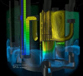
Figure 5.11. Multiscale thermo-hydraulic calculations of a 4th generation reactor core (source: calculation performed with the CA THARE system^ code, the Trio-MC core code and the TrioCFD CFD code – ©CEA/Direction de l’Énergie Nucléaire). For a color version of this figure, see www.iste.co.uk/sigrist/simulation2.zip
COMMENT ON FIGURE 5.11.– The code architecture for understanding and simulating the thermohydraulics of reactor cores has been designed to develop as generic a tool as possible. The development of the tools is the result of the collaboration of many experts: physicists, mathematicians and engineers who work together to validate development choices.
They combine various approaches that make it possible to report on global fluid circulation phenomena, as well as finer flow models in the vicinity of the various components of the reactor.
“Turbulent phenomena come into play in the thermohydraulics of reactors. However, the finest models, such as provided in LES simulation (representing large eddies in turbulence), are not necessary in all areas of the reactor: simulations span different approaches, which is more efficient! The challenge is then to make different flow models (1D, 2D or 3D) coexist with different turbulence models. Expertise that is collectively held by different experts…”
5.3.3. Developing nuclear fusion
Fusion is the nuclear reaction that feeds our Sun and is an almost inexhaustible source of energy. With a very low impact on the environment, its control would be a response to many of humanity’s energy needs in the 21st Century… and beyond? It occurs in plasmas, the environment in which light elements can combine and produce energy. Plasma is sometimes presented as the fourth state of matter. These environments are found, in particular, within the stars (Figure 5.13).
A fusion plasma is obtained when a gas is heated to extreme temperatures in which the electrons (negatively charged) are separated from the nuclei of the atoms (positively charged). Experimental devices aim to artificially recreate conditions on Earth that are favorable to fusion reactions. In particular, magnetic confinement fusion plasma is a tenuous environment, nearly a million times less dense than the air we breathe.

Figure 5.13. The energy of the Sun and stars comes from the fusion of hydrogen
(source: www123rf.com/rustyphil)
COMMENT ON FIGURE 5.13.– What we perceive as light and heat results from fusion reactions occurring in the core of the Sun and stars. During this process, hydrogen nuclei collide and fuse to form heavier helium atoms – and considerable amounts of energy. Not widely distributed on Earth, plasma is the state under which more than 99.9% of the visible matter in the Universe occurs. There are different types of plasmas: cold (to a few hundred degrees) or very hot, dense (denser than a solid) to thin (more diluted than air). The core plasmas of magnetic confinement fusion machines are thin (about 100,000 times less dense than ambient air) and very hot (about 150 million degrees). In the core of stars such as the Sun, fusion occurs at much higher densities (about 150 times that of water) and at temperatures about 10 times lower (source: www.iter.org).
The temperature is such that it partially overcomes the repulsion forces opposing different charge particles and thus allows the material to fuse. The ITER machine, for example, is one of these: its objective is to control fusion energy. Involving 35 countries (those of the European Union, the United States, India, Japan, China, Russia, South Korea and Switzerland), it is one of the most ambitious global scientific projects of our century3. It is a step between the research facilities that preceded it and the fusion power plants that will follow it.
The Cadarache site in France, near the CEA center, has been hosting ITER facilities since 2006. It should host a first plasma in 2025 and carry out controlled fusion reactions by 2035. ITER is a “tokamak”, a Russian acronym for a magnetized toroidal chamber: the conditions conducive to fusion are obtained by magnetic confinement (Figure 5.14).
In a tokamak, the particles have a helix-shaped trajectory around the magnetic field lines that wind around virtual interlocking toroidal surfaces. The temperature in the plasma core is in the order of 10–20 kilo-electron-volts (keV) – these are extremely high values, with 1 keV representing more than 10 million degrees Celsius! It falls to a few eV (1 eV corresponds to about 11,000 °C) near the walls of the tokamak.
Yanick Sarazin, a physicist at the CEA’s Institute for Research on Magnetic Containment Fusion, explains one of the challenges of current fusion research:
“The gigantic temperature differences between the reactor core and the walls make the plasma of the thermodynamic systems ‘out of balance’. They naturally tend to approach a situation of thermal equilibrium by dissipating the heat within them: we speak of ‘relaxation’. Turbulence in the plasma contributes significantly to these heat losses. One of the objectives of the tokamak design is to force the organization of turbulence, so that relaxation takes place slowly. It is, among other things, under these conditions that fusion performance will be economically viable”.

Figure 5.14. Obtaining a plasma in a device: example of the European JET “tokamak” before and during its operation (source: www.iter.org). For a color version of this figure, see www.iste.co.uk/sigrist/simulation2.zip
COMMENT ON FIGURE 5.14.– Three conditions must be met to achieve fusion in the laboratory: a very high temperature (to cause high-energy collisions), a high plasma particle density (to increase the probability of collisions) and a long containment time (to maintain the plasma, which tends to expand, in a defined volume). The fusion reaction can be obtained in a machine using very intense magnetic fields to confine and control the hot plasma: the giant ITER coils thus deliver fields of a few tesla, nearly a million times the Earth’s magnetic field (source: www.iter.org).
Numerical simulation is the tool of choice for researchers to understand the origin of turbulence in tokamaks – and to predict and control it in order to limit heat loss. Plasma physics is fundamentally described by the equations of Magneto-Hydro-Dynamics (MHD), which can be seen as the coupling between the Navier-Stokes (Box 2.1) and Maxwell equations (Chapter 2 of the first volume). Unfortunately, three-dimensional numerical simulations of the MHD are insufficient to describe the turbulent heat transport processes in these highly diluted and very low collision environments.
The researchers then work with kinetic models based on the Boltzmann equation, already discussed in Chapter 2. The calculations focus on the evolution of the charged particle distribution function, which measures the probability of finding them in a given volume of 6-dimensional “phase space”. The phase space is made up of the three position variables and three particle velocity components – in practice, an additional assumption reduces the problem to five components of the phase space, whose evolution over time is monitored.
The characteristic flow quantities (mass, amount of movement, energy, etc.) are obtained by calculating the weighted averages of the distribution function. The resolution of kinetic equations coupled with Maxwell equations is based on different methods:
- – Lagrangian methods consist of calculating the distribution function as a result of the dynamics of microparticles, whose interaction, described with the Newton equation, defines their trajectory. This method is well suited to parallel calculation but has its limits in the case of turbulent flows, where trajectories become chaotic and are more difficult to calculate. This can lead to a loss of information in some regions of the phase space. This results in “numerical noise”: disrupting calculations, it can nevertheless be reduced by dedicated techniques;
- – Eulerian methods consist of calculating the distribution function on a fixed grid of the phase space, using discretization methods as described in Chapter 1 of Volume 1. It makes it possible to comply, more accurately, with the conservation conditions but loses its effectiveness when implemented in a parallel computer.
An intermediate method, called Arbitrary Lagrange-Euler or ALE, encountered in Chapter 2 concerning fluid-structure interactions (Box 2.2), is adapted to the resolution of MHD equations in the Boltzmann statistical formalism, by separating the resolution of flow equations, treated in an Eulerian manner at the current time step, and electromagnetic equations, treated in a Lagrangian manner at the previous time step.
Virginie Grandgirard, a computer scientist at the CEA’s Institute for Research on Magnetic Containment Fusion, details the difficulties encountered in the simulations:
“Even with the most efficient numerical methods, such as the ALE approach, simulations are constantly limited by computational means. GYSELA, the calculation code developed at the CEA to simulate turbulence in tokamaks, uses the largest French and European computers: a complete simulation of the physical phenomena we want to study requires nearly a week of calculation on 16,000 to 32,000 processors!”

Figure 5.15. Simulation of turbulence developing in a tokamak. For a color version of this figure, see www.iste.co.uk/sigrist/simulation2.zip
COMMENT ON FIGURE 5.15.– The simulation represents an instant map of the turbulent structures calculated in a tokamak plasma, visualizing the electrical potential. Carried out with the GYSELA code, developed at the CEA center in Cadarache, France, the simulation makes it possible to visualize how the eddies stretch along the magnetic field lines [GRA 16]. It helps researchers understand the dynamics of turbulence in tokamak plasma and how it influences heat transfer (source: Yanick Sarazin and Virginie Grandgirard, Office of the Commissioner for Atomic Energy and Alternative Energies).
HPC calculation (Chpater 3 of the first volume) is therefore a crucial tool to support researchers in their understanding of fusion physics. In order to remove the technical obstacles posed by the control of tomorrow’s nuclear energy, it will be necessary to change the scale in the power of the computers. The quest for the Exascale has only just begun, and because of its strategic nature for fusion control, the GYSELA code is one of the tools used by the European EoCoE-II project – which aims to support the porting of the calculation codes used by the energy communities to the exa-flop ECU class. The adaptation of a calculation code to such computers requires the collaboration of experts from different disciplines: theoretical and applied physicists, computer scientists, simulation experts, code developers and users. The energy of the 21st Century will also depend on the fusion of multiple scientific skills!
5.4. New energies
Driven by an awareness of ecological issues, the search for alternative energy sources – wind, waves, sun, heat from the sea, land or waste – as opposed to carbon and uranium continues to grow (Figure 5.16).
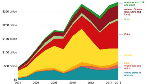
Figure 5.16. Global investment in renewable energy (source: Our World in Data/https://ourworldindata.org/renewables). For a color version of this figure, see www.iste.co.uk/sigrist/simulation2.zip
COMMENT ON FIGURE 5.16.– In 2004, global investments in renewable energy amounted to $47 billion, reaching $286 billion by 2015, an increase that could be seen in all regions of the world, albeit at different levels. The largest increase was in China: from $3 billion in 2004 to $103 billion in 2015, investment in China increased more than 30-fold – compared to the global average of 7 billion. China is nowadays the most significant investor in renewable energy, with its financial capacity representing that of the United States, Europe and India combined.
5.4.1. Hydroelectricity
In the Chinese city of Fengjie, on the Yangtze River, a man and a woman meet in search of their past. A past that the city will engulf, once submerged by the gigantic Three Gorges Dam. With his film Still Life, Chinese filmmaker Ja Zhang-Ké tells a nostalgic story, whilst questioning the meaning of the long march of Chinese economic development [ZHA 07]. It is set against the backdrop of the construction of one of the largest civil engineering structures of our century (Figure 5.17).
Located in the mountainous region of Haut-Yangzi, the 2,335-m-long and 185-m-high Trois-Gorges dam came into service in 2009, after more than 15 years of construction. Its electricity production covers less than 5% of China’s energy needs, the world’s largest hydropower producer ahead of Canada, Brazil, the United States and Norway – countries crossed by many large rivers and streams and thus benefiting from an abundant resource.
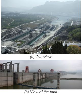
Figure 5.17. The Three Gorges Dam
(source: www123rf.com)
COMMENT ON FIGURE 5.17.– A hydroelectric power plant consists of a water intake or reservoir, as well as a generating facility. Over the distance between the dam and the power plant, water passes through a canal between the intake and return points, a gallery or penstock. The greater the difference in height, the greater the water pressure in the plant and the greater the power produced. The amount of energy is proportional to the amount of turbinated water and the height of fall. The Three Gorges Dam reservoir stores nearly 40 billion m3 of water, the equivalent of 10 million Olympic swimming pools, and covers more than 1,000 km2, the equivalent of 100,000 football fields. The waterfall height, about 90 m, represents a discharge capacity of more than 100,000 m3/s. The capacity recovered by the 30 turbines of the Three Gorges Dam amounts to 22,500 MW, seven times the capacity of the Rhône hydroelectric power stations (in France), estimated at 2,950 MW.
The energy transported by the flow is recovered by means of turbines (Figure 5.18), a device invented at the dawn of the 20th Century by French engineers Claude Burdin (1788–1873) and Benoît Fourneyron (1802–1867). Exploiting their patent and improving their invention, the French engineer Aristide Bergès (1833–1904) created, in 1882, one of the first electricity production plants on the Isère River in France.

Figure 5.18. Francis turbine (1956), at the leading edges of cavitation-eroded blades
(source: www.commons.wikimedia.org)
Since their first use, turbines have been constantly adapted to the applications for which they are intended by engineers. The current machines are designed to meet the challenges of renewable energy. Guillaume Balarac, a researcher in fluid mechanics and their applications to hydraulics, explains:
“The energy produced by exploiting certain renewable resources is intermittent and hydropower is increasingly required to be able to absorb the fluctuations in solar and wind power production. As a result, hydroelectric turbines are operating at new speeds far from their nominal design points. Marked, for example, by large fluctuations in hydraulic loads or low loads, flows in these regimes are often very unstable and characterized by complex physical phenomena, such as turbulence or cavitation”.
Cavitation develops when the pressure drops below the threshold where the gases dissolved in the fluid remain compressed. As when opening a bottle of champagne, bubbles are formed that affect the flow characteristics and efficiency of the turbine. Very unstable, these bubbles can also implode by releasing a significant amount of energy into the liquid. The shockwave resulting from the implosion then becomes sufficient to damage solid surfaces. As a result, cavitation erosion (Figure 5.18) is a major concern for turbine or propeller designers, significantly reducing their service life.
“Numerical simulation allows us to understand the new operating modes of turbines and helps to broaden their operational ranges. The appearance of eddies, or cavitation, clearly modifying the efficiency of the turbines, the models aim to accurately represent the physics of flows, and in particular, turbulence. Statistical methods, deployed in the average modeling of Navier-Stokes equations (RANS), have their limitations here. The calculations are based on large-eddy models (LES), which are much more representative of turbulent dynamics and the pressure fluctuations they generate”.
With large-scale simulations, researchers and engineers are better able to predict flow trends. By more precisely analyzing the causes of yield loss with the calculation, they can also propose new concepts or optimize existing shapes [GUI 16, WIL 16]. Calculations require fine mesh sizes to be able to capture physical phenomena on a small scale (Figure 5.19) and restitution times increase proportionally.
LES models produce a large amount of data, in particular the velocity and pressure at each point and at each time step of the calculation. This information is then used to analyze the flow, using statistical quantities (average velocity and pressure, and the spatial and temporal fluctuations of these fields, turbulence energy, etc.), close to those that an experiment would provide. These are obtained at the cost of long calculations, sometimes lasting a few months! The complete simulation of a turbine using LES models is still not possible, so calculations focus on the machine body. In order to account for the flow conditions at the turbine inlet, they are based on experimental data, or calculated using less expensive methods, such as in RANS method.

Figure 5.19. Mesh size used for LES simulation of a turbine body [DOU 18]. For a color version of this figure, see www.iste.co.uk/sigrist/simulation2.zip
COMMENT ON FIGURE 5.19.– The figure shows the mesh used to simulate flow around a turbine blade with LES modeling. The first calculation, performed on a 4 million cell mesh, has a low spatial resolution and does not capture vortex formation in the vicinity of the blade. Based on a mesh size of nearly 80 million cells, the second one has sufficient resolution to finely simulate the flow. LES calculations remain very expensive in terms of modeling, calculation and analysis time. For industrial applications, they are often used in conjunction with RANS models. Taking advantage of near-wall RANS models and LES models in regions further away from them, DES (Detached Eddy Simulation) methods make it possible, for example, to accurately represent flows in the presence of obstacles, at more accessible calculation times than LES models can offer [CAR 03].
While these LES calculations are not yet industrially applicable, they provide valuable guidance to turbine designers:
“With LES models, for example, we have identified areas of high energy dissipation due to instabilities in observed flows for vertical axis turbines. In an attempt to reduce the formation of these turbines, we have proposed a new design for these turbines through simulation…”
5.4.2. Wind energy
Recovering the energy contained in the wind is the challenge that engineers are also trying to meet: offshore wind energy, for example, is developing in various regions of the world and various projects are being developed. The preferred locations for installing farms are those with good wind conditions (Figure 5.20).
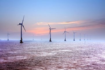
Figure 5.20. Offshore wind turbine fields
(source: www123rf.com/Wang Song)
COMMENT ON FIGURE 5.20.– A wind turbine is a turbine set in motion by the forces exerted by a flow on its blades. The shape of these is designed to separate the air flow and accelerate it differently depending on the face of the blade profile: the more strongly accelerated flow exerts a lower pressure on the profile than the less accelerated flow. This pressure difference generates a driving force on the blades and sets them in motion. The mechanical energy due to their rotation is then converted into energy made available on an electrical grid. The power theoretically recoverable by a wind turbine depends on air density, blade size and flow velocity. For a horizontal axis wind turbine, the theoretically recoverable power is proportional to the square of the diameter of the turbine and the cube of the wind speed. The largest onshore wind turbines, whose diameter is generally between 130 and 140 m maximum, develop powers in the range of 2–4 MW; offshore wind turbines, with a larger diameter (typically between 160 and 180 m), deliver a nominal power in the range of 6–8 MW depending on wind conditions.
Horizontal axis wind turbines are nowadays much more widespread than vertical axis wind turbines. The latter are a potentially preferable solution to the former in two niche sectors:
- – urban environments, because they behave better in changing and turbulent wind conditions;
- – the marine environment, as they can have interesting characteristics for floating wind turbines. In a vertical axis wind turbine, the electricity generator can be placed close to the water level, which facilitates maintenance operations, and the center of gravity is lower, which improves the stability of the floating structure.
Vertical axis wind turbines operate at generally reduced rotational speeds, which can lead to “dynamic stall” under certain conditions. Similar to a loss of lift for an aircraft wing, it involves more complex, highly unsteady and intrinsically dynamic physical phenomena for this type of wind turbine: in particular, a release of eddies interacting with the blades is observed. These phenomena result in a significant decrease in the wind turbine’s efficiency.
Numerical simulation provides a detailed understanding of the nature of air flows, and helps to anticipate the risks of boundary layer detachment in low velocity flow regimes. Laurent Beaudet, a young researcher and author of a PhD thesis on the simulation of the operation of a wind turbine [BEA 14], explains:
“My work has helped to improve numerical models for predicting detachment for a vertical axis wind turbine. I have developed a calculation model based on the so-called ‘vortex method’. This allows any type of simulation of load-bearing surfaces, such as helicopter blades, wind turbines, etc., to be carried out and to represent these surfaces and the vortex structures developing in their wake. Potentially applicable to various wind turbine concepts, it is a particularly interesting alternative to 'traditional' CFD calculation methods, such as deployed in RANS or LES simulations, in terms of calculation costs in particular”.
This method is becoming increasingly important in the wind energy sector, with different types of applications for which it is effective:
“In order to support the development of increasingly large and flexible offshore wind turbines, it is necessary to couple an advanced aerodynamic calculation module with a structural dynamics solver and a controller. The analyses of wind turbine load cases, necessary for their certification, are based on such ‘multi-physical’ models. For these simulations, representing both the flow, motion and deformation of the blades, and the actuators/motors of the wind turbine, optimizing the calculation times is crucial and the vortex method meets this need”.

Figure 5.21. Flow calculation around a vertical axis wind turbine (source: Institut P’/https://www.pprime.fr/). For a color version of this figure, see www.iste.co.uk/sigrist/simulation2.zip
COMMENT ON FIGURE 5.21.– The figure illustrates the simulation of a vertical axis wind turbine (the “Nov’éolienne”, developed by Noveol), using a vortex method, implemented in the GENUVP calculation code (GENeral Unsteady Vortex Particle code). This tool, originally developed by the National Technical University of Athens (NTUA), allows aerodynamic simulations for a wide variety of configurations and applications. The models used for this type of calculation have a wide scope and are of interest to many applications. It should be noted that vertical axis wind turbines have not yet reached sufficient maturity and reliability to be able to be deployed en masse – in particular their service life remains very limited because they are subject to high fatigue stresses.
A capricious resource, wind exhibits great variations in speed, time and space. This disparity conditions the investments required for farm projects, both at sea and on land, or the installation of wind turbines in urban areas. The power delivered by a wind turbine varies greatly for wind speeds between 3 and 10 m/s, and reaches an almost constant value above 10 m/s. In this interval, the slightest fluctuation in speed can result in significant yield losses and the task of wind project engineers is to find the siting areas where wind speed is the highest and turbulence the lowest. Stéphane Sanquer, Deputy General Manager of Meteodyn, explains:
“Site data is essential in the design of a wind power project. They are usually obtained by dedicated devices, such as a measuring mast. The operation of such instrumentation being very expensive, it is generally impossible to base a site analysis on this method alone. Numerical simulation makes it possible to complete in-situ measurements. To this end, we have developed an ‘expert tool’, dedicated to wind simulations on complex terrain (mountainous, forest, urban areas, etc.). Calculations allow a relationship to be established between the data from on-site measurements at a given point and any other point on the site. Based on information on the measurement point, wind statistics in ‘average meteorological’ conditions, or more exceptional conditions (such as storms), the simulation reconstructs the corresponding mapping over the entire fleet”.

Figure 5.22. Wind measurement mast on a wind site
(source: Le Télégramme/https://www.letelegramme.fr)
Proposing a global approach to the wind power project [CHA 06, DEE 04, LI 15], the calculation methodology is based on:
- – an implementation database. This describes in particular the land cover, i.e. the roughness and characteristics of the terrain, which have a major influence on local wind conditions;
- – a solver for flow equations (stationary Navier–Stokes model). The latter report on turbulence and thermal effects using models specific to atmospheric physics.
Based on the finite volume method, the solver uses efficient numerical methods: a calculation for a given wind direction requires a few hours on “standard” computer resources. A complete wind mapping, exploring different cases of interest to engineers, is thus obtained in a calculation time compatible with the schedule of a project;
- – a module for analyzing the calculation results. It is carried out according to specific criteria, useful to engineers and adapted to wind energy projects (such as average or extreme values of wind speeds, energy production over a given period and on given areas of the site).

Figure 5.23. Evaluation of a site’s wind resource (source: calculation carried out with the MeteoDyn/WT6 software by the company MeteoDyn/www.meteodyn.com). For a color version of this figure, see www.iste.co.uk/sigrist/simulation2.zip
The calculations provide additional expertise to the measurements and contribute to a better estimation of the performance of the future installation. Ensuring the production of a wind farm is a crucial element and simulation has become one of the key elements in the development of a wind energy investment plan. The development of wind turbine farms poses many technical challenges, including understanding the interaction between a wind turbine’s wake and its neighbors and the yield losses it causes. In order to study such phenomena, researchers and engineers implement complex flow simulations, using dedicated methods, hybridizing mean turbulence models (RANS) or large-scale turbulence models (LES).
The uses of numerical simulation in the field of energy, of which we have given some examples in this chapter, cover a large number of applications and problems – they extend in particular to buildings, with the aim of saving resources, reducing energy losses or evaluating the effects of sunlight (Figure 5.24).

Figure 5.24. Evaluation of the effects of sunlight on an urban area using dynamic thermal simulations (source: www.inex.fr). For a color version of this figure, see www.iste.co.uk/sigrist/simulation2.zip
COMMENT ON FIGURE 5.24.– The “dynamic thermal simulation” of a building is the study of the thermal behavior of a building over a defined period (from a few days to 1 year) with an hourly, or lower, time step. The modeling aims to account for all parameters affecting the heat balance, such as internal and external heat inputs, building thermal inertia, heat transfer through walls, etc. Models describing thermal phenomena require knowledge of geometric data (such as wall thickness, shape of thermal screens, etc.) and material characteristics (such as coefficients describing their ability to store or propagate heat). Dynamic thermal simulation makes it possible to estimate the thermal requirements of buildings in operation, taking into account, for example, the various thermal inputs and the behavior of the occupants and the local climate. Among the external thermal inputs, sunlight receives particular attention from architects, design offices, etc. The simulation can then be used to design buildings according to different criteria (minimize or maximize solar gains or seek optimal protection) and supports their energy optimization.
As emphasized in Chapter 3 of Volume 1, numerical simulation is somehow an energy-consuming technique. However, examples given in this chapter also suggest that it has gradually become a major asset to tackle challenges in all energy sectors. It opens now to new application areas, such as biomechanics.
- 1 X-rays are emitted during electronic transitions, the passage from one energy level to another by an electron. Becquerel discovered gamma rays, resulting from the disintegration of atoms, which were explained in 1919 by the English physicist Ernest Rutherford (1871–1937). X and gamma rays are two electromagnetic waves, emitted at different frequencies (Figure 2.15 of the first volume).
- 2 In fact, no mode of energy production really is, when taking into account extraction, transformation and of primary sources (hydrocarbons, uranium), building and maintenance of production sites (refinery, power plant), waste management, etc.
- 3 Initially acronym of International Thermonuclear Experimental Reactor, ITER nowadays refers to the Latin word for “path” – designating the way to be followed by scientists working to control nuclear fusion energy?