
1
Agriculture
In 1916, Chicago, Bill was a worker employed in a foundry. Following an altercation, he fled the city, accompanied by his girlfriend Abby and his sister Linda. He found refuge in Texas where wheat was harvested from huge arable areas and a favorable climate allowed him to grow it. Hired as a seasonal worker by a wealthy farmer suffering from an incurable disease, Bill pushed Abby to give in to his employer’s advances. A calculation to get out of poverty? Set in a bourgeois house drowned in an almost endless expanse of wheat, inspired by the paintings of the American painter Andrew Wyeth (1917–2009), Days of Heaven (1978) recounts a psychological drama [MAL 78]. The contemplative camera of its author, the American filmmaker Terence Malik, also depicts the blazing sun of long working days, the power of harvesting machines and the hazards of harvests, stormy bad weather or locust invasion, which become a tragedy subject to the whims of the sky – whose unpredictability symbolizes that of human passion?
Controlled and perfected for more than 10,000 years, as attested to by remains from ancient Egypt (Figure 1.1), agriculture remains a survival challenge for a humanity facing climate change in the 21st Century even though it is capable of changing its practices.
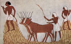
Figure 1.1. Cereal harvest, Tomb of Menna, Sheikh Abd el-Gournah Necropolis, Egypt
(source: 10,000 Meisterwerke der Malerei, The Yorck Project)
1.1. Feeding the world
Agriculture is also at the center of current ecological concerns and strategic issues, particularly those of state food sovereignty, to which simulation techniques provide answers. Today, the world’s cultivated land covers more than 50 million km2 (Figure 1.2): this area is about three times that of Russia, the largest country in the world with 17 million km2.
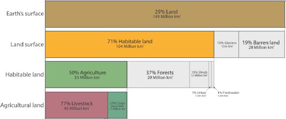
Figure 1.2. Allocation of land areas for food production (source: Our World in Data/https://ourworldindata.org/yields-and-land-use-in-agriculture). For a color version of this figure, see www.iste.co.uk/sigrist/simulation2.zip
COMMENT ON FIGURE 1.2.– Only 30% of the total area of our planet is covered by land, 70% of which is considered habitable (about 100 million km2). Humans use about half of it for agriculture, and less than one-tenth for urban infrastructure. More than three-quarters of the agricultural land is used for animal husbandry, combining land allocated to pasture and feed production (these aggregate data obviously do not reflect disparities between countries).
The share of cultivated land has grown steadily for more than 10,000 years to meet the needs of a constantly growing world population. The latter was estimated at less than 1 billion people at the beginning of the 19th Century, reaching nearly 7 billion at the beginning of the 21st Century. In 2015, the four most populous countries in the world were China (1.4 billion), India (1.3 billion), the United States (305 million) and Brazil (201 million). Demographic projections estimate a world population of more than 11 billion people in 2100 (Figure 1.3).

Figure 1.3. World population growth between 1750 and 2015 and projections to 2100
(source: Our World in Data/https://ourworldindata.org/world-population-growth)
COMMENT ON FIGURE 1.3.– Since the 1970s, humanity as a whole has been undergoing a demographic transition. The growth of the world population is the result of the combined effects of births and deaths. It is marked by a significant increase that commenced at the beginning of the 20th Century. It peaked at more than 2% in 1973 and has since declined to 1.2% in 2015. Demographic projections estimate it at 0.1% by 2100. Behind this global representation are significant differences between countries. Poverty is the first factor delaying the demographic transition: the world’s least wealthy countries are also those with the highest population growth.
The productive capacity of each country (Figure 1.4) depends on soil quality, the area available or used for agriculture, the climatic conditions to which it is exposed and the available cultivation techniques and agricultural practices developed there. While people’s lifestyles are very disparate and partly reflect the wealth of nations, humanity as a whole lives on credit, consuming resources at a faster rate than the Earth can provide.
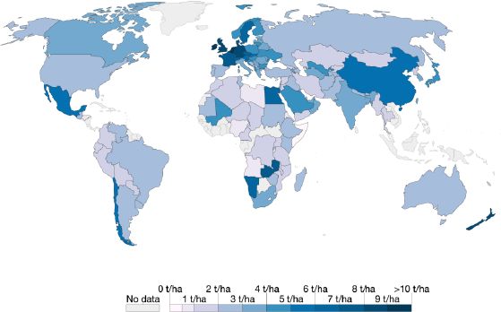
Figure 1.4. Annual world wheat yields for 2014, expressed in tons per hectare. Wheat is the primary cereal produced in the world, aimed at both human and animal consumption (source: Our World in Data/https://ourworldindata.org/yields-and-land-use-in-agriculture). For a color version of this figure, see www.iste.co.uk/sigrist/simulation2.zip.
The American non-governmental organization Global Footprint Network calculates the Earth Overshoot Day each year. The latter corresponds to the date of the current year on which humanity is supposed to have consumed all the resources that the planet is capable of regenerating in 1 year. One of the pieces of data derived from this NGo’s calculations is the number of planets Earth that would be needed to meet humanity’s consumption of renewable resources in 1 year. By 2018, 1.7 planets Earth are needed to support humanity – and the extrapolation of the data shows that the threshold of two planets Earth will be exceeded well before the end of the first half of the 21st Century.
Yet, in many Western countries, consumption and production patterns lead to a significant waste of food resources and production (Figure 1.5), showing that humanity has real room for maneuver to change its relationship with the wealth of resources that the planet that hosts it still offers.
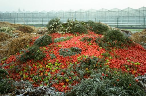
Figure 1.5. Although edible, these tomatoes, produced in France, are discarded because they do not meet certain criteria based on the standardization of production and their packaging (source: © Jacques Péré, from the series “La Beauté du diable”, exhibition at the Galerie Lyeux Communs, Tours, June 2018). For a color version of this figure, see www.iste.co.uk/sigrist/simulation2.zip.
COMMENT ON FIGURE 1.5.– Nearly one-third of the food produced annually worldwide (1.3 billion tons) is destroyed or wasted. The leading position is occupied by fruits and vegetables. The amount of food lost every year is equivalent to more than half of the annual cereal production. Waste is higher in rich countries, where consumers throw away as much food each year as sub-Saharan Africa produces at the same time (more than 220 million tons). Food waste is observed at all stages of the food chain and concerns all actors: 32% is attributed to agricultural production, 21% to processing, 14% to distribution, 14% to collective and commercial catering and 19% to home consumption (sources: www.fao.org,www.ademe.fr).
From the resources they consume, those from agriculture are among the most important for humans and the most strategic for States. During the 20th Century, advances in agricultural technology as a whole have generally reduced famine episodes whose causes are attributable to yield collapse [PIN 18b]. They have also been accompanied by irreversible environmental destruction, for example when new areas are being sought for intensive cultivation through massive deforestation.
All over the world, some farmers are trying to renew current agricultural practices. Their credo is that more sober techniques can give as good results as those of intensive agriculture in particular, which consumes a lot of energy and water (Figure 1.6), and whose excesses are also increasingly contested [SOL 19].
“Nature has so much real wealth to unveil and humans have such a definitively superior potential for intelligence, that the combination of the two frankly gives hope […] Working with nature and not against it, we realize that the solutions are there, before our eyes and that they often prove to be simpler and less costly in energy […] We have divided by thirty our energy efficiency to produce food since the time of our grandparents… that sounds like a terrible insult to human intelligence” [ROS 18].

Figure 1.6. How thirsty is our food?
(source: https://www.statista.com/chart/9483/how-thirsty-is-our-food/)
COMMENT ON FIGURE 1.6.– We use water in any productive activity, the amount consumed depending on two main factors: the climate of the production region and the agricultural practices developed there. For example, 35 L of water is needed to produce a cup of tea, 140 L for a cup of coffee, 75 L for a glass of beer and 120 L for a glass of wine; 2,400 L are consumed for the production of a hamburger, 40 L for a slice of bread and 13 L for a tomato (source: www.fao.org).
In the 21st Century, will numerical modeling contribute to the development of agricultural techniques that ensure a sufficient level of agricultural production for all humanity and limit the degradation of its environment?
1.2. Agriculture is being digitized
In the richest countries, agriculture is becoming digital and modeling is a key focus of this change [WAL 18]. David Makowski, an expert in this field at INRA*, explains the objective:
“Germany, Australia, France, Italy, the United States and the Netherlands are the pioneering countries in the use of numerical modeling in agriculture, recently joined by China. Numerical simulation makes it possible to assess the impact of agricultural practices, soil quality and climate on yields and the environment. The applications are varied and allow farmers, companies and public agencies to estimate the performance of different production methods in different situations. Despite the sometimes significant uncertainty of their simulations, models are frequently used to predict the environmental impact of agriculture by assessing the emissions of particulate matter, greenhouse gases or pollutants due to agricultural practices”.
Numerical simulations in agronomy have used “mechanistic models” for two to three decades. These allow the functioning of crops to be described by means of equations; these, for instance, represent the production of biomass as a function of solar radiation, or the growth of plants as a function of soil temperature or humidity. Simulations make it possible to account for the physiological and biological dynamics of plants, on the scale of a plot or a set of cultivated lands. They can represent different agricultural practices and help to assess their impact on yields.
An example of modeling applicable to biological phenomena? The interaction model between hosts and biological control auxiliaries. It describes how biological populations, such as predators and their prey (aphids and ladybirds for example), evolve in an ecosystem. For example, it explains the development cycles of many species (animal, plant, etc.) in many environments, such as the marine phytoplankton (Figure 1.7).
The model consists of two differential equations, proposed independently by two mathematicians, the Austrian Alfred-James Lotka (1880–1949) and the Italian Vito Volterra (1860–1940), in 1925–1926. These equations are written as:

The equations describe the evolution of the prey and predator population, represented by variables x(t) and y(t). The first equation states that prey, having access to an unlimited source of food, would grow exponentially (this is rendered by the first term in the right-hand side of the equation αx(t)), and are sometime faced with predators at certain occurrence (this is rendered by the second term of in the right hand side of the equation –βx(t)y(t)). The second equation states that predators perish from natural death (this is rendered by the first term in the right-hand side of the equation –α′x(t)), but grow by hunting prey (this is rendered by the second term of in the right-hand side of the equation +β′y(t)x(t)).

Figure 1.7. Satellite image showing algae growth in a North Atlantic region (source: www.nasa.gov). For a color version of this figure, see www.iste.co.uk/sigrist/simulation2.zip
COMMENT ON FIGURE 1.7.– In the waters of the North Atlantic, a large amount of phytoplankton, microscopic algae that play a role in the food chain of the marine ecosystem and contribute to the ocean carbon cycle, develops each spring and fall. The image is a photograph taken by NASA’s “Suomi” satellite on September 23, 2015. Blue spirals represent high concentrations of algae, waters loaded with microscopic creatures that contribute to the production of part of the planet’s oxygen.
The Lotka–Volterra equations have as unknown the populations of the competing species, the coefficients describe their survival and mortality rates. They predict a cyclical evolution of populations that is consistent with the observations (Figure 1.8). Many other equation-based models are available for studies of organic and agricultural systems. In recent years, data-based simulations have been developed to complement these models – nowadays, they use methods such as automatic learning techniques, discussed in Chapter 4 of the first volume. Statistical models are based on an adjustment of equations to data and allow an empirical relationship between different quantities to be established.

Figure 1.8. Typical evolution of the prey/predator populations as predicted by the Lotka-Volterra equations
Satellites, drones (Figure 1.9), sensors, field surveys: statistical models are based on a large number of data and it is the variety and diversity of the latter that gives credibility to predictions. Data used in statistical models are diverse: they describe the crop environment (e.g. topography and meteorology), farmers’ practices (e.g. frequency of watering or spreading), animal species behavior or plant species growth.

Figure 1.9. Agricultural drones are used to monitor crops and collect useful data to develop or validate certain simulations
(source: © Christophe Maitre/INRA/www.mediatheque.inra.fr/)
The models of each family complement each other, each providing information whose multimodel analysis makes it possible to identify trends [MAK 15]:
“Modeling is a synthetic expertise of the knowledge available to a community at a given time. One of the most promising approaches is to reconcile these classes of models with the statistical processing of simulation data. The efficiency and reliability of ‘Big-Data’ techniques is increasing, and it is not excluded that they may eventually replace models based on equations…”.
Simulations involve equations coupling different scales (plant, plot, farm or agricultural region). They require a large amount of data and still require very long computational times. Despite these current limitations, which artificial intelligence algorithms help to push back, modeling in agriculture is becoming more widespread and a tool for scientific debate and political decisions. Let us listen to the researchers involved in the development of models through a few examples.
1.3. Decision-making support
Farmers, political and economic decision makers, and consumers shape the landscape of agricultural practices to varying degrees, each acting at its own level: by guiding a continental agricultural policy, by deciding to invest in a new machine tool, or simply by doing one’s shopping. Different agents, actors and practices influence it and the behaviors of each have societal and environmental consequences.
Some agricultural practices have potentially negative impacts on climate and biodiversity, for example [BEL 19]. The disappearance of many insect species is attributed to the destruction of their habitat by intensive agriculture and their poisoning by the widespread use of pesticides [HAL 17, SAN 19]. How can these harmful effects be anticipated and limited? How can climate change be taken into account in current and future practices [BAS 14]? What is the best combination of agricultural practices that makes it possible to produce while guaranteeing a country’s food sovereignty? How can we legislate and cultivate for the benefit of the greatest number of people? Hélène Raynal, researcher at INRA and project manager of a digital platform dedicated to agrosystems [BER 13] provides an initial answer:
“Different models aggregated within a shared computer system make it possible to represent agricultural systems taking into account their complexity. Modeling should be able to represent biological processes, such as plant growth. They must also make it possible to account for physical processes related, for example, to water (evaporation of water from the soil, drainage of water to the deep layers of the soil, etc.), carbon and nitrogen, which are the factors that determine agricultural production. They must also integrate the climate dimension or farmers’ practices (such as irrigation levels), and socio-economic aspects. These processes fit into different scale levels and, depending on the issue, the model is used to simulate a cultivated field, an agricultural operation – or even an entire region. The aim is to integrate as much relevant information as possible into the model, from soil chemistry to local climate factors, agricultural practices and assumed market trends or climate changes. Simulations make it possible to play on various scenarios and estimate the impact of a decision taken by stakeholders in the sector on agricultural production. They can also help to design new agricultural systems adapted to different issues, such as climate change and the reduction of chemical inputs to the crop”.
This collaborative platform1 offers various services for the construction and computer simulation of models. In particular, it offers a range of mechanistic models produced by agronomists. Based on mathematical equations, they explain the biophysical and chemical phenomena involved in crop growth, the effects of bioaggressors or model economic balances. They are built separately by specialists in these different fields [RAY 18].
“In an overall simulation, it is a question of coupling different scales of description and reporting changes over time at the desired frequency (day, month, year), as well as in heterogeneous territories. When simulations aim to secure public actions, they focus on the country’s overall production. It is necessary to have a set of calculation points representing the different practices, which change according to the soil, the size and type of farms, the varieties grown and, of course, the weather conditions. Having data available to feed the models is a key point in the simulations”.
The complexity of the different models used in interaction in a simulation leads to rather long calculations: performed on dedicated IT infrastructures, an overall simulation requires 2 days full of calculations and generates several gigabytes of data. The researchers’ experimental design is limited to half a dozen situations used to generate data for subsequent analyses.
Scientists develop global indicators, reflecting the state of the system: they include soil quality, the yield of the territories observed (plot, farm and region), water (consumed, drained or irrigated) and nitrogen (consumed, drained or generated) cycles. Additional simulations on targeted areas allow the results to be refined. Together, they contribute to estimating the dynamics of the simulated systems, characterizing their agronomic interest and their environmental and economic sustainability (Figure 1.10). In some cases, simulation can help inform public decision-making, such as assessing the consequences of a public policy decision.
The same approach can be replicated at the farm level to inform farmers’ choices. Combining compliance with environmental standards and profitability, some production systems are efficient and unknown to some farmers who may, for various reasons, hesitate to adopt them.
Christophe and Stéphane Vigneau-Chevreau are two winegrowers from the Loire Valley [SIG 19]. They cultivate parcels of vines of about 30 hectares in the Vouvray appellation. When taking over the family farm, founded in 1875 and run by four generations before them, more than 20 years ago, they decided to convert it to organic farming. It is becoming necessary and obvious for them to stop using pesticides, which alter the soil in its ability to regenerate and deliver all its minerals necessary for viticulture:
“For the treatment of classic vine diseases, we use contact products sprayed on the grapes and eliminated with water, without altering the grain or taste of the wine. Unlike phytosanitary products, which impregnate the sap of the vine and are found… even in the glass! In addition, the use of pesticides depletes the soil: to compensate, it is then necessary to use artificial yeasts during vinification, which erases the aromas and uniqueness of the soil”.

Figure 1.10. Share of production allowed by the ecosystem services associated with grain maize cultivation [THE 17]. For a color version of this figure, see www.iste.co.uk/sigrist/simulation2.zip
COMMENT ON FIGURE 1.10.– This map, based on simulation results, shows that for grain maize cultivation, about half of the annual input requirements of plants are provided by ecosystem services and therefore fertilizer inputs could be limited. The simulation work is part of the EFESE study (Évaluation française des écosystèmes et des services écosystémiques). Launched in 2012 by the French Ministry of the Environment, the study aims to provide knowledge on the current state and sustainable use of ecosystems.
The transition from their farm to the AB label, which warrants organic farming practices, was done at the cost of intense work:
“The first three years, we gradually adapted our plots; this was accompanied by a drop in yield that was not immediately offset by an increase in quality. It took us about ten years to ensure a quality and performance that we consider satisfactory!”
More than 20 years ago, this mode of production was not understood. At the beginning of the 2000s, it became a guarantee of quality and consumers were not mistaken, meeting the offer proposed by the two brothers and by other producers in their region. Their bet proved to be a win–win situation for all.
Models developed by researchers in digital agriculture can support the decision and transition required by such reconversions (Figure 1.11). Hélène Raynal explains:
“Models contributing to decision-making are a delicate matter. They reproduce, at the farm level, the calculations made, for example, for the whole country in the context of public policies. Including detailed data – such as the equipment available for irrigation or exploitation, crop organization and location on the land, possible polyculture rotations, cohabitation with livestock, etc. In addition, the models also seek to capture farmers’ preferences: the risks they are willing to take in their investments, the balance they want to favor between short- and long-term productivity, the time they spend at work and how they can integrate environmental issues”.
Simulations are carried out on the plots and make it possible to develop an overview of everyone’s practices. By enriching them with climate change data, they offer farmers the opportunity to anticipate some of their consequences in the long term.
“The criteria for analyzing simulation data are developed with the farmers involved in the process: this joint approach is essential to ensure its relevance and quality. While the most traditional indicators are those of investments and returns, operators also include those of quality of work, such as the possibility of taking days off… This criterion is, for example, a determining factor in the choices of certain operators – and it is highly contextual”.
Many professionals are on the lookout for new practices and the models proposed by researchers give them the means to make profitable decisions.

Figure 1.11. Working hours (per ha and per year) required by a farmer for “conventional” agricultural production (yellow squares) and pesticide-free production (orange triangles), as part of a durum wheat and sunflower crop rotation, in southwest France [RAY 17]. For a color version of this figure, see www.iste.co.uk/sigrist/simulation2.zip.
1.4. Environmental impact
Fertilizers are organic substances, of plant or animal origin, or mineral substances (synthesized by the industrial fixation of atmospheric nitrogen) intended to provide plants with nutrient supplements. They contribute to improving their growth and increasing the yield and quality of production.

Figure 1.14. Fertilizers promote plant growth but their overintensive use has long-term harmful effects on the environment or may be dangerous for human health
(source: www.123rf.com/)
COMMENT ON FIGURE 1.14.– Often used in a mixture, fertilizers are mainly composed of three elements: nitrogen contributes to the vegetative development of all overground parts of the plant, phosphorus strengthens their resistance and participates in root development, and potassium promotes flowering and fruit development. They also provide plants with complementary elements (such as calcium or magnesium) and trace elements (such as iron, manganese, sodium or zinc), useful for plant life and development. Their use dates back to the early days of agriculture and, nowadays, the development of the chemical industry encourages their use, sometimes to an excessive extent.
Their widespread use worldwide (Figure 1.15) supports the yields expected by some farmers, often at the expense of soil, water and air quality. Used in excessive quantities, fertilizers are responsible for the depletion, or even destruction, of ecosystems – inhibiting the ability of soils to regenerate naturally or permanently polluting groundwater reserves.

Figure 1.15. Global use of nitrogen, potassium and phosphate fertilizers worldwide in 2014: major agricultural countries are making massive use of fertilizers. The quantities used are expressed in kilograms per hectare of cultivated land (source: Our World in Data/https://ourworldindata.org/fertilizer-and-pesticides). For a color version of this figure, see www.iste.co.uk/sigrist/simulation2.zip.
Sophie Genermont, a researcher at INRA, has been working for more than 20 years on the development of a platform for simulating ammonia emissions resulting from the use of fertilizers [GEN 97, RAM 18], which contribute to the degradation of air quality:
“Formed from organic nitrogen, ammonia is a pollutant of the air, and after deposition, of soils and water. About 95% of anthropogenic ammonia (present in the environment through human action) comes from agriculture.
My work on the formation and volatilization of this compound is based on data measuring its concentrations in plants, water or soil. These are complemented by models of the physical, physico-chemical and biological processes at different scales”.
The platform developed because of the work carried out over more than 20 years by various research teams is initially dedicated to liquid organic manure. Its functionalities are extended in order to apply the modeling to mineral fertilizers [CAD 04] and thicker organic fertilizers [GAR 12], and to study pollution due to the use of certain plant protection products [BED 09]. It is also used to assess the consequences of certain livestock practices – which are also responsible for high nitrogen emissions [SMI 09].
Models are carried out for a plot, a small agricultural region, a country, or even, in the long term, a continent! They take into account the various factors that influence the migration of ammoniacal nitrogen in the environment – and exploit the data that make it possible to characterize it: meteorological, geological variables for the composition of surface soils, physical and chemical variables for the composition of fertilizers, statistics for the input practices carried out by farmers.
“The simulations consist in solving equations modeling the physical, physicochemical and biological phenomena at work in soils, and at the interface between the soil and the atmosphere. Carried out on a plot scale, they give very fast results: a few seconds of calculation give an idea of the evolution of the phenomena that can actually be observed over a few weeks and this at an hourly time step!”
A set of simulations, aggregated for different plots and taking into account composition differences as well as meteorological factors, allows data to be reproduced on larger scales – typically a small agricultural region.
“It is possible to scale up, for a country, with the same principle: by performing as many simulations as necessary to describe an entire region and synthesize the results of the calculations. No less than 150,000 simulations are needed to represent the use of mineral and organic fertilizers during the soil fertilization phase (in the fall and then from February to late spring) and estimate their effects on the scale of a country like France. Two days of calculation on about forty cores are necessary to realize it!”.
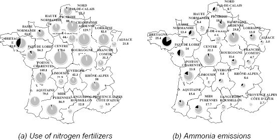
Figure 1.16. From the use of nitrogen fertilizers to ammonia emissions in France [HAM 14]
COMMENT ON FIGURE 1.16.– The figure on the left represents the quantities of nitrogen used in agriculture in France during the 2005–2006 crop year in the form of ammonia and urea and therefore susceptible to volatilization (the values are expressed in thousands of tons of ammoniacal nitrogen). The figure on the right shows the resulting ammonia emissions (values are expressed in thousands of tons of ammonia, NH3). The choice is made here to present the results of the calculations for the entire season, according to the different regions of the country and for the two main categories of fertilizers: synthetic fertilizers (in gray) and organic waste products (in black).
The difficulty of the calculation lies in the reliability of the data required to inform the model: composition of the fertilizers used, types of fertilized soil, crop species and the fertilization routes preferred by farmers, including dates, doses and forms of fertilizer applied and methods of application.
“Simulations allow us to identify interesting trends. Their quality depends very much on the quality of the data on which they are based. Soil type, range of inputs, emission data and field surveys are the preferred sources for researchers to inform their models. The validation of the calculations continues to pose problems: although the simulations are able to report the concentration of ammonia in the air with good spatial and temporal resolution, we do not currently have such an accurate measurement network to directly compare the results of our calculations with field observations – this is a current area of research involving different teams in France”.
The researchers’ calculations tend to reflect the variability of the situations encountered through sensitivity studies: their analyses are being refined and are providing decision-makers with tangible evidence for assessing the risks associated with the massive use of fertilizers and, in the near future, phyto-pharmaceuticals.
1.5. Plant growth
Vegetation is one of the crucial resources for humanity, providing it with food and energy – and in some cases a place to live. Satellite observations help to consolidate plant occupancy data on the planet’s surface (Figure 1.19). They enable scientists to understand the influence of natural cycles on vegetation (such as droughts or epidemics) or that of human activities (such as deforestation or CO2 emissions).
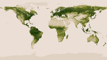
Figure 1.19. Vegetation map obtained from satellite observations (source: NASA/www.nasa.gouv). For a color version of this figure, see www.iste.co.uk/sigrist/simulation2.zip
COMMENT ON FIGURE 1.19.– The shades of green on the map correspond to values ranging from 0.0 to 1.0, in arbitrary units. Values close to 1.0 (dark green) indicate the presence of abundant vegetation, as in the Amazon rainforest. Values close to 0.0 (beige) indicate areas with little vegetation, such as the oceans or the Arctic continent. Forests cover 30% of the world’s land area, equivalent to just under 40 million km2, while treeless vegetation (tundra, savannah, temperate grasslands) occupies about the same area.
In 1985, English filmmaker John Boorman recounted in The Esmerald Forest how a world disappears, the world of the Amazon rainforest tribes [BOO 85]. The son of an engineer who oversees the construction of a gigantic dam is taken from his parents by a tribe of Forest Men. As the dam’s construction was completed, the father and son found themselves in circumstances that led them both to confront progress and humanity. The dam will eventually give way under the waters of a river doped by torrential rain, engulfed by the songs of frogs calling on the forces of nature. The engineer who wanted to destroy his work to protect the future of his son and that of a tribe wishing to live in peace will not have this power.
The Amazon rainforest is still one of the largest plant communities on the planet today. According to FAO2 estimates, it is now disappearing at an average rate of 25,000 km2 per year (equivalent to half the size of Austria) to make way for new crops. At this rate, it will have completely disappeared by the first half of the next century. It pays the highest price for the consequences of human activities: more than half of the world’s deforestation. The evolution of vegetation as a whole is of particular concern because of its dual importance: it supports a large part of biodiversity and contributes to the absorption of atmospheric CO2. Analyzing satellite observation data, NASA researchers show that in just under 20 years, the planet has re-vegetated with an area equivalent to that of the Amazon, with India and China being among the main contributors to this trend. The observed vegetation corresponds, on the one hand, to the growth of new forests, contributing to the sequestration of carbon from the atmosphere, and, on the other hand, to an extension of agricultural areas, whose natural carbon storage balance is generally neutral [CHE 19].
Understanding the growth mechanisms of species continues to occupy scientists. In the first half of the 20th Century, the British biologist d’Arcy Thompson (1881–1946) became interested in the shape and growth of living organisms, publishing his thoughts in an exciting collection [THO 61]. He looks for invariants and universal principles that govern the evolution of life – for example, fractal structures or particular sequences (Figure 1.20).

Figure 1.20. The Fibonacci spiral: a model (too simple?) to explain plant growth
(source: www.123rf)
COMMENT ON FIGURE 1.20.– Leonardo Fibonacci (1170–1250) was a 13th Century Italian mathematician. The Italy of his time was a region formed by scatterings of merchant cities in strong competition (Venice, Pisa, Genoa). Trade activities needed numbers and calculation to support their economic development. The mathematician developed algebraic methods to contribute to this. In particular, he drew inspiration from Indian and Arab mathematics, while Roman numerals, still widely used in Europe, forced calculation in a rigid numbering system that the invention of zero helped to loosen. The sequence that bears his name is defined from two values, then each term is calculated as the sum of the two previous ones. Thus, starting from 1 and 1, the terms are 2, 3, 5, 8, 13, 21, etc. This sequence, which has properties of interest to mathematicians, is found in some natural growth mechanisms. The Fibonacci sequence hides the famous golden number ![]() Discovered in the 3rd Century BC by Greek mathematicians, Φ seems to be present behind the architectural choices made in antiquity, for example in the construction of the Parthenon in Greece. “Let no one ignorant of geometry enter” is the motto of the Academy, founded in Athens by Plato in the 4th Century BC. The Platonic school makes mathematics one of the instruments of the search for truth. To this is added that of harmony, whose golden number is the hyphen. Φ is the Greek letter traditionally used to designate it and it also refers to philosophy. For very different reasons, the golden number fascinates human beings who sometimes tend to find it everywhere even where it is not [LIV 02].
Discovered in the 3rd Century BC by Greek mathematicians, Φ seems to be present behind the architectural choices made in antiquity, for example in the construction of the Parthenon in Greece. “Let no one ignorant of geometry enter” is the motto of the Academy, founded in Athens by Plato in the 4th Century BC. The Platonic school makes mathematics one of the instruments of the search for truth. To this is added that of harmony, whose golden number is the hyphen. Φ is the Greek letter traditionally used to designate it and it also refers to philosophy. For very different reasons, the golden number fascinates human beings who sometimes tend to find it everywhere even where it is not [LIV 02].
Created at the initiative of the Royal Botanical Garden of Edinburgh, the website The Plant List3 aims to provide an exhaustive list of the various plant species: there are currently more than 1 million. Nature is characterized by a great variability of shapes (Figure 1.21): how can we accurately model the development of such diverse plants?

Figure 1.21. Variety of leaf shapes
(source: www.123rf/Liliia Khuzhakhmetova)
Since the late 1960s, scientists have been using a formalism that is particularly well suited to modeling plant growth. It finds its roots not in the field of mathematics but in that of grammar! Frédéric Boudon, a researcher at CIRAD*, is an expert in these tools, the so-called “L-systems”:
“The L-systems were introduced in the late 1960s by Hungarian biologist Aristid Lindenmayer to describe some of the processes encountered in biology. They are particularly effective in modeling plant development and are based on the rules of ‘formal grammar’. These can provide a realistic account of the influence of the plant’s architecture, vitality and environment on its growth”.
In an L-system, a plant is represented by a sentence whose elements, or modules, themselves symbolize the components of the plant (stem, branch, flower, leaf, etc.). A set of rules governs the dynamics of these modules: they formalize biological processes and model plant transformations. The production of a new element (leaf, flower, fruit), growth or division of an existing element (stem, branch) are therefore represented by sentence equivalents of our language, which itself has its own syntactic rules (the order of words in a sentence) and is based on a given semantics (a set of words).
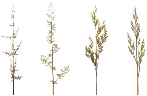
Figure 1.22. Weeds generated by a three-dimensional L-system program
(source: www.commons.wikimedia.org)
COMMENT ON FIGURE 1.22.– The rules implemented in the L-systems seek to represent the living: the probability of regrowth of a cut part, the amount of biomass produced, the birth and hatching of a flower, the production and ripening of a fruit. They can take into account environmental factors: amount of light received, level of sugar reserves, concentration of a hormone, etc. They make it possible to arrive at a very realistic modeling, a genuine digital plant!
“The validation of models is done by comparing them with the dynamics and patterns observed in the field. There are no specific restrictions on the use of L-systems and researchers can therefore treat any type of plant: grasses, plants, trees! Their architectures can be reproduced in a very realistic way, including at fine detail levels. By using so-called ‘stochastic approaches’, it is possible to reproduce by simulation the heterogeneity observed in nature. Different biophysical phenomena such as branch mechanics or their reorientation towards the sun or as a function of gravity can be included in these simulations”.
While they formalize the understanding of plant growth through simple mathematical rules, L-system-based models allow different types of applications such as yield prediction. The challenge in this case is to have models interact at different scales in order to obtain an overview: from plants or planting groups, to the plot and the entire farm. This is a vast field of research in digital agriculture. Modeling by L-systems already contributes to the evaluation of certain techniques, such as agro-ecology, which are receiving increasing interest due to the growing awareness of ecological issues and the need to preserve the emerald forest?
Let us conclude this chapter with the understanding that, in general, agricultural modeling addresses three scientific issues:
- – understand and predict plant growth processes;
- – assess the impact of agricultural practices in ecological and economic terms;
- – informing the policies of decision makers and farmers’ choices.
They are thus becoming an essential tool for agricultural research, meeting the vital needs of humanity in the 21st Century: feeding populations and preserving their environment.
- 1 Available at: https://www6.inra.fr/record.
- 2 Data available at: http://www.fao.org/forestry.
- 3 Available at: http://www.theplantlist.org/.