
6
Stability of Linear FDEs Using the Nyquist Criterion
6.1. Introduction
In this chapter, we present a frequency technique for the stability analysis of linear differential systems, either with integer order or fractional order derivatives; moreover, these systems can include time delays.
Fundamentally, a linear ordinary differential equation (ODE) (i.e. with integer order derivatives) is stable if the roots of the characteristic polynomial are not situated in the right half complex plane (RHP). Obviously, the stability problem can be solved by calculating these roots. Historically, mathematicians and control engineers preferred techniques avoiding this calculation. Two families of methods, based on the complex variable theory [LEP 80], are available: the Routh–Hurwitz criterion [ROU 77, HUR 95] and the Nyquist criterion [NYQ 32].
Based on polynomial properties, the Routh–Hurwitz criterion indicates the number of RHP roots of the characteristic polynomial (or unstable poles of the ODE) owing to relations between the coefficients of this polynomial. From a practical point of view, this criterion is easy to use, but its proof is difficult to establish [HAN 96]. Moreover, for a stable ODE, it does not quantify its stability degree.
The Nyquist criterion basically deals with closed-loop systems. Based on a curve in the complex plane representing the graph of the open-loop transfer function and on a contour including the RHP, it indicates the number of unstable poles of the closed-loop transfer function. This criterion is easy to use (especially in its simplified version) and relatively easy to prove using the complex variable theory [LEP 80, GIL 90]. Moreover, it allows the quantification of the stability degree of the closed-loop (at the origin of robust design techniques); on the contrary, it does not apply to systems in open-loop.
The stability of nonlinear ODEs is analyzed with another approach, the Lyapunov technique [LYA 07, LAS 61, KRA 63]. Fundamentally, it is connected to the state space model of the differential system: this system is stable if a particular function of the state variables, representing its “energy”, is decreasing when there is no external excitation.
Although these three techniques are very classical, it is interesting to recall them in order to situate the stability of fractional differential equations (FDEs) (i.e. with fractional order derivatives) in a general framework.
First of all, similarly to the integer order case, the stability of linear FDEs relies on the hypothesis that the roots of their characteristic polynomial are not situated (see Chapter 7 of Volume 1) in the RHP [OUS 95a, BON 00]. Basically, FDEs are infinite dimensional systems; thus, the number of roots of their polynomial is also infinite: stability analysis by calculation of these roots is not a simple task in the general case [DAS 13]. Moreover, the usual stability results rely on a restrictive modeling of FDEs: the basic hypothesis deals with commensurability, i.e. the fractional derivative orders have to be an integer multiple of a minimal fractional order. Thanks to this hypothesis, some stability results are available, mainly based on Matignon’s theorem [MAT 98, SAB 08a]. On the contrary, despite some interesting results [RAP 15, RAP 16], the case of non-commensurate order FDEs remains an open problem.
The case of time-delayed differential systems has long been investigated with integer order derivatives [DUG 97, NIC 97, RIC 03]. Two main approaches can be considered, the first one being derived from the Routh–Hurwitz criterion, and the second one from the Lyapunov technique. Because the characteristic polynomial includes time delays, the number of its roots is infinite. Stability analysis is based on frequency techniques, which indirectly determine the number of unstable roots by a generalization of the Routh–Hurwitz criterion [NIC 97]. The Lyapunov approach uses an extended quadratic function of the state variables, according to a principle formulated by Krasovskii [KRA 63]. The case of linear FDEs with time delays remains an open problem, with some existing results, such as the works of [HOT 98, BON 00, HWA 06].
Fundamentally, our approach is based on a closed-loop principle for any kind of system governed by a linear ODE or FDE [TRI 09c, MAA 09, SAB 13].
This closed-loop principle [BEN 08a] is derived from the analysis of the analog simulation scheme of any differential system in the controller canonical form [KAI 80]. This simulation scheme reveals a true closed-loop system, whose stability corresponds to the stability of the considered ODE or FDE. Thus, system stability can be analyzed using the Nyquist criterion.
With this methodology, it is possible to give an alternate demonstration of the Routh-Hurwitz criterion for ODEs, besides with a quantification of the stability degree. In the case of FDEs, it is possible to generalize ODEs results, however, with a severe limitation due to the complexity of analytical results. The stability of time-delayed differential systems, either based on ODE or FDE models, can also be analyzed with this approach, which appears to be very general. Moreover, it is important to note that no particular modeling is required in the definition of FDEs.
After a recall of FDE definitions and simulation methodology, the principle of the stability technique is presented in section 6.2. This method is applied to ODEs in section 6.3 and to FDEs in section 6.4; it is generalized to ODEs with time delays in section 6.5, and finally to FDEs with time delays in section 6.6.
6.2. Simulation and stability of fractional differential equations
6.2.1. Simulation of an FDE
Consider the general linear FDE whose transfer function is
The fractional differentiation orders
are real positive numbers; they are called external or explicit orders. It is necessary to define internal or implicit derivation orders such as (see Chapter 1 of Volume 1):
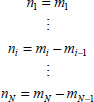
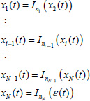
The classical controller canonical state space form [KAI 80] is presented in Figure 6.1 with

and
6.2.2. Stability of the simulation scheme
The simulation diagram in Figure 6.1, which exhibits a direct transfer composed of integration operators Ini (s) and a feed-back signal r(t) composed of the sum of the weighted states ai – 1xi(t), with the error signal ε(t) = u(t) – r(t), explicitly refers to a closed-loop system, which is necessarily subject to a stability condition.
Of course, the stability condition of this feedback system corresponds to the stability of the differential system characterized by the transfer function ![]() i.e. to the stability condition of the considered FDE.
i.e. to the stability condition of the considered FDE.
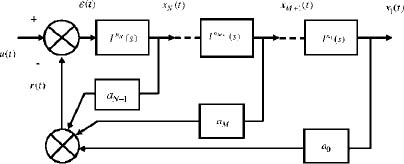
Figure 6.1. Closed-loop simulation of an FDE with fractional integrators
These considerations are not new: analog computer users were perfectly aware of this stability problem (see Chapter 1 of Volume 1) which became implicit with digital computers.
Consequently, the explicit formulation of this simulation stability problem, with an open-loop transfer function HOL(s), provides a method for the stability analysis of H(s) using the Nyquist criterion [NYQ 32, GIL 90].
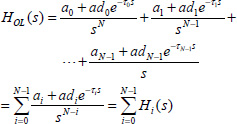
Let us define HOL(s) as
where
Some elementary calculations provide
It is easy to verify that
and thus
The well-known term 1+ HOL (s) explicitly refers to the stability of a closed-loop system, although H(s) corresponds to an open-loop FDE (or ODE).
6.2.3. Stability analysis of FDEs using the Nyquist criterion
As the previous simulation scheme refers to a closed-loop system with an open-loop transfer function HOL (s), it is possible to analyze the stability of the considered FDE (or ODE) using the Nyquist criterion [NYQ 32, GIL 90]. Strict application of the Nyquist criterion is based on the definition of a D contour in the RHP. First of all, it is important to note that HOL(s) has only poles in s = 0; the particular form of HOL (s) excludes unstable poles. Thus, the contour has to be modified to exclude the poles in s=0.
Then, with this modified D contour (see Figure 6.2), the net number of rotations of HOL(s) around the (–1 + j 0) point (critical point) is strictly equal to the number of unstable poles of H(s) in the RHP.

Figure 6.2. D contour excluding the origin
If the FDE or ODE is stable (see Figure 6.3), this net number of rotations is equal to zero, i.e. if HOL(s) does not encircle the critical point (see [BEN 08a] for more details with FDEs).
The application of the generalized Nyquist criterion provides the number of unstable poles (see Chapter 7 of Volume 1).
Nevertheless, if we are only interested in the stability of the FDE, a simplified version of the Nyquist criterion can be used. It can be formulated as: if the Nyquist diagram HOL (jω), plotted from ω = 0 to ω →+∞, is situated on the “right side” of the critical point (–1 + j 0), then the system H(s) (or the FDE) is stable; else it is unstable.
Moreover, the distance between the Nyquist diagram and the critical point provides information on the stability degree (phase and gain margins) of the FDE (ODE).

Figure 6.3. Example of the Nyquist contour for a stable ODE
6.3. Stability of ordinary differential equations
6.3.1. Introduction
The principle of the stability analysis based on the Nyquist criterion is exposed thanks to a third-order ODE example. First, it is necessary to define the general open-loop transfer function and to present the technique used to draw its approximate Nyquist graph
6.3.2. Open-loop transfer function
Let us define
which is the transfer function of a Nth -order linear ODE.
It is interesting to note that we obtain this transfer function from the model of the general FDE with N derivatives [6.1, 6.3] simply by imposing
According to Lord Kelvin’s principle [THO 76], the simulation of this ODE requires N integrators ![]() .
.
As with an FDE, we obtain a closed-loop system where the active elements are the N integrators and the an parameters. The bm parameters have no effect in this closed-loop: as it is well known, this means that the stability of H(s) depends only on the transfer ![]() .
.
Thanks to the principle previously presented, HOL(s) transfer function can be expressed as
It is straightforward to verify that
and
6.3.3. Drawing of HOL(jω) graph in the complex plane
The objective is to present a technique to draw an approximate graph of HOL(jω).
HOL(s) is composed of N terms such as ![]() , i.e. of N directions
, i.e. of N directions ![]() in the complex plane.
in the complex plane.
Let us define
then
and
where
The corresponding graph is a ray centered at the origin and characterized by the polar angle θi. Since θi is an integer multiple of ![]() , these rays coincide with the real or imaginary coordinate axes.
, these rays coincide with the real or imaginary coordinate axes.
The graph of HOL(jω) is the combination of these N elementary graphs.
It is important to note that two of these directions are asymptotes:
- – if ω → 0, then HOL (jω) behaves like the higher power element in ω, i.e.
which is the low frequency asymptote.
- – if ω → ∞, then HOL (jω) behaves like the lower power element in ω, i.e.
which is the high frequency asymptote.
Thus, the graph of HOL(jω) is constrained by these two asymptotes: this is a simple way to draw an approximate graph of HOL (jω).
6.3.4. Stability of the third-order ODE
6.3.4.1. Definition
Let
Then
The two asymptotes are
and
If a0, a1 and a2 are positive coefficients, the corresponding approximate graph of HOL(jω) is presented in Figure 6.4.
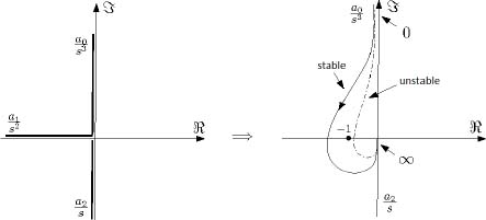
Figure 6.4. Open-loop graph of a third-order ODE
6.3.4.2. Stability condition
The stability condition can be deduced from the simplified Nyquist criterion, based on the position of HOL(jω) graph relatively to the critical point (–1 + 0j).
Let us define
with
The ODE is at the limit of stability if the HOL(jω) graph is on the critical point.
The condition X = –1 provides
(oscillation frequency) whereas Y = 0 provides the parameter condition for oscillation
According to Figure 6.4, the system is stable if
This leads to
which is of course the stability condition provided by the Routh-Hurwitz condition [ROU 77].
Moreover, it is interesting to note that the graph of HOL(s) in the Nichols chart provides the stability margins, i.e. information on the dominant poles of H(s) (see Figure 6.5).
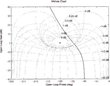
Figure 6.5. Nichols chart of the third-order ODE
6.3.4.3. Complete stability criterion
The Routh-Hurwitz criterion indicates that H(s) is stable if all the an parameters are strictly positive with a0 < a1a2.
Is it possible to obtain all these conditions with the proposed approach?
Of course, the Nyquist criterion is able to give a satisfactory answer to this question.
For example, consider the a1 parameter and the graphs in Figure 6.4. If a1 = 0, the graph of HOL (jω) is situated on the imaginary axis, and H(s) is unstable.
If ![]() and HOL(jω) graph are in the RHP; thus, H(s) is unstable.
and HOL(jω) graph are in the RHP; thus, H(s) is unstable.
The case of the a0 parameter is interesting.
Consider a0 < 0 : it is necessary to apply the complete Nyquist procedure in this case to obtain all the pertinent information.
The complete graph of HOL(s) in the complex plane is obtained using the excluding contour in the RHP (see Figure 6.2). With this contour, we obtain the graph presented in Figure 6.6. The closed-loop curve representing HOL(s) encircles the critical point only once: this means that H(s) has only one unstable pole. This pole is necessary real; thus, the corresponding impulse response is divergent.
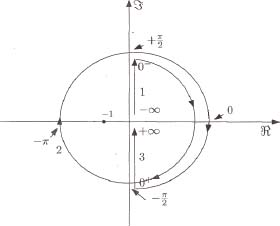
Figure 6.6. Open-loop Nyquist’s graph of the third-order ODE
6.3.5. Conclusion
The application of the proposed approach to ODEs provides the same results as the Routh–Hurwitz criterion. A particular feature of this methodology is that it is mainly graphical: we exhibited, with the third-order ODE example, the importance of the HOL(jω) approximate graph constructed on the basis of directions in the complex plane. Thus, the proofs of stability are obviously more simple to demonstrate than with the Routh-Hurwitz technique [HAN 96].
However this simplicity does not exclude rigor if necessary: the application of the complete Nyquist procedure provides all necessary information, for instance the number of unstable poles.
Moreover, the graph of HOL(jω) in the Nichols chart makes it possible to quantify the stability degree of the ODE, which is a supplementary information compared to the simple Routh–Hurwitz approach.
6.4. Stability analysis of FDEs
6.4.1. Introduction
The stability of FDEs with one and two derivatives is investigated. Some analytic results for systems with N fractional derivatives are given, and a general numerical approach is proposed.
6.4.2. Drawing of HOL(jω) graph in the complex plane
HOL(jω) given in [6.8] is the sum of N elementary terms such as
Let us define
Then
and
As described previously, the corresponding graph is a ray centered at the origin, characterized by the polar angle θi. The difference with the ODE case is that the values of θi are fractional multiples of ![]() .
.
The graph of HOL(jω) is the combination of these N elementary graphs.
Two directions are also asymptotes
- – If ω → 0, then HOL(jω) behaves like
which is the low frequency asymptote.
- – If ω → ∞, then HOL(jω) behaves like
which is the high frequency asymptote
As in the ODE case, HOL(jω) is constrained by these two asymptotes: this is a simple way to draw an approximate graph.
Consider for example the graph of Figure 6.7 where all the ai parameters are positive.

Figure 6.7. Open-loop approximate graph
6.4.3. Stability of the one-derivative FDE
Let us consider the system
with one fractional derivative.
The stability results for this simple system are well known [OUS 95a]; therefore, it is interesting to compare them with our approach. In this case
and
with

As N = 1, HOL(jω) is composed of only one ray characterized by the polar angle
The graph of HOL(jω) is presented in Figure 6.8 for different values of n with a0 > 0.
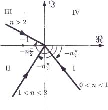
Figure 6.8. Open-loop graph of the one-derivative FDE
The simplified Nyquist criterion indicates that the system is unstable for n ≥ 2. Obviously, this result can be established analytically. The stability limit corresponds to
The condition Y = 0 implies
which is obtained with n = 2.
The condition X = –1 provides the oscillation frequency
The system remains stable if
Thus,
which leads to n < 2.
When a0 is negative, it is preferable to use the complete Nyquist criterion. Using the excluding contour of Figure 6.2, the corresponding graph of HOL(s) is presented in Figure 6.9 for 0 < n < 1.

Figure 6.9. Open-loop Nyquist’s graph of the one-derivative FDE
As HOL(s) encircles the critical point only once, H(s) has a real pole in the RHP, and the system is unstable by divergence (see Chapter 7 of Volume 1).
Thus, we can conclude as follows.
If a0 > 0:
- – for 0 < n < 1, the system is stable and aperiodic;
- – for 1 < n < 2 , the system is stable and underdamped oscillatory;
- – for n = 2, the system is unstable and has two poles on the imaginary axis;
- – for 2 < n < 3, the system is unstable and has two poles in the RHP.
If a0 < 0, the system is unstable and has one real pole in the RHP.
6.4.4. Stability of the two-derivative FDE
6.4.4.1. Definitions
Let us consider
with
In this case
The graph of HOL(jω) is the combination of two directions:
- – a low frequency asymptote
- – a high frequency asymptote
6.4.4.2. Graphical analysis of stability
Consider a0 > 0 and a1 > 0 with 0 < n1 < 1, 0 < n2 < 1 and n1+n2 > 1, we obtain the graph presented in Figure 6.10.
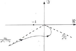
Figure 6.10. Open-loop graph of the stable FDE
Of course, we can conclude that H(s) is stable.
With 0 < n2 < 1 and 2 < n1 + n2 < 3, we obtain the different graphs presented in Figure 6.11.
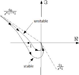
Figure 6.11. Open-loop graph of the conditionally stable FDE
In this case, the system is conditionally stable.
REMARK 1.– It is important to note that these results have been obtained with an elementary graphical approach.
6.4.4.3. Stability condition
Let
with
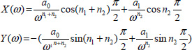
The stability limit corresponds to X = –1 and Y = 0. The condition Y = 0 provides the oscillation frequency
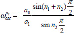
Since ![]() is necessarily positive, it implies that
is necessarily positive, it implies that
Finally, putting ωosc in X = –1, we obtain the parametric condition between, a0, a1, n1 and n2, i.e.

The system (with a0 >0, a1 >0) remains stable if Y<0 when X = –1 or equivalently
Using one of these two conditions, we can analytically calculate the inequality that a0, a1, n1, n2 have to verify.
REMARK 2.– Note that when a0 > 0 and a1 < 0, the condition ![]() is fulfilled with 0 < n1 + n2 < 2.
is fulfilled with 0 < n1 + n2 < 2.
REMARK 3.– With ODEs, only the ai parameters have an influence on stability. On the contrary, with FDEs, the fractional orders ni also have an influence on stability, which can be discussed graphically.
As an example, consider the case
When n1 =2, the low frequency asymptote is opposite to the high frequency one, as presented in Figure 6.12. The graph of HOL(jω) is situated on this common line: the system is unstable.
When n1 > 2, the graph of HOL(jω) is situated in the upper sector corresponding to the two asymptotes (see Figure 6.13) and the system is unstable.

Figure 6.12. Instability caused by n1 = 2

Figure 6.13. Instability caused by n1 > 2
This analysis can be generalized to n2, and thus we obtain a fundamental result stated as follows: the fractional system H(s) is unstable ∀ni ≥ 2.
6.4.4.4. Example
Consider the case a0 > 0 and a1 < 0: with a second-order ODE, this value of a1 leads to instability. However, with an FDE, the stability depends on the respective values of n1 and n2.
Consider 0 < n1 < 1 and 0 < n2 < 1: as a1 < 0, the direction ![]() reverses and the corresponding graph is presented in Figure 6.14.
reverses and the corresponding graph is presented in Figure 6.14.
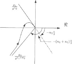
Figure 6.14. Two-derivative FDE with a1 > 0
Obviously, the stability is conditional in this case.
Consider n1 = n2 = 0.5, the oscillation frequency is provided by:
We deduce that
when H OL(jω) = –1.
Moreover, stability is ensured if
Consider a1 = –1, the stability is ensured by
For a0 = 0.7, we present the corresponding Nichols chart in Figure 6.15 and the step response in Figure 6.16.
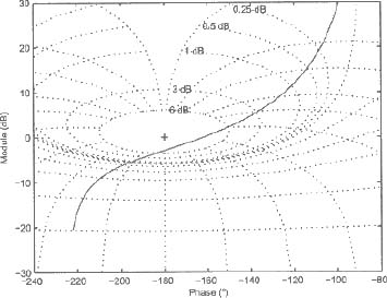
Figure 6.15. Nichols chart with a0 = 0.7
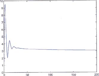
Figure 6.16. Step response with a0 = 0.7
We can note that it is possible to quantify the damping of the step response, thanks to the stability margins in the Nichols chart.
Finally, for a0 = 0.4 , we verify that the system is unstable: see the step response in Figure 6.17.
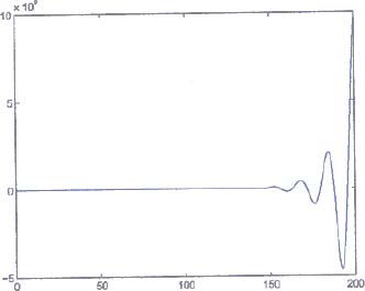
Figure 6.17. Step response with a0 = 0.4
6.4.4.5. Conclusion
We can summarize the following stability conditions for the two-derivative FDE, obtained graphically or analytically:
If a0 < 0, H(s) is unstable (as noted previously).
If a0 > 0 and a1 > 0
- – for 0 < n1 + n2 < 2, the system is unconditionally stable;
- – for 0 <n1 < 2 and 0 < n2 < 2 with n1+ n2 > 2, the system is conditionally stable;
- – for n1 ≥ 2 or n2 ≥ 2, the system is unstable.
If a0 > 0 and a1 < 0
- – for 0 < n1 < 1 and 0 < n2 < 1, the system is conditionally stable;
- – for 0 < n1 < 1 and 1 < n2 < 2, the system is conditionally stable;
- – for 1 < n1 < 2 and 0 < n2 < 1, the system is conditionally stable;
- – for 1 < n1 < 2 and 1 < n2 < 2, the system is unstable.
6.4.5. Stability of the N-derivative FDE
Finally, we consider the general transfer function [6.1]. It is difficult to provide general results due to the difficulty of the analytical calculations. However, it is possible to give some general rules, as the following one obtained graphically. The graph of H OL(jω) is constrained by the two asymptotes already presented in Figure 6.7. Consider the case
then the low frequency asymptote is situated under the real axis, and the system is unconditionally stable.
Therefore, we can formulate some simple rules:
- – if a0 < 0, the system is unstable;
- – if ai > 0 ∀ i and
 , the system is unconditionally stable;
 - – if ai > 0 ∀ i and ni > 2 ∀ i, the system is unstable.
However, despite the lack of analytical results, it is always possible to numerically analyze the stability with the proposed frequency approach. The drawing of HOL(jω) in the Nichols chart gives essential information on system stability and on its stability degree thanks to the stability margins.
6.4.6. Conclusion
We demonstrated that the proposed approach to system stability applies to non-commensurate order FDEs, generalizing the Routh-Hurwitz criterion. Based on the Nyquist criterion approach, it provides information concerning stability, number of unstable poles and degree of system stability.
Another important feature of this method is its graphical interpretations, which provide very simple demonstrations.
Despite the complexity of analytical formulations in the general case, this method can be numerically implemented with any linear fractional system, providing information on its stability and its degree of stability.
6.5. Stability analysis of ODEs with time delays
6.5.1. Introduction
The previous technique is applied to time-delayed systems. Therefore, it is necessary to test its ability to analyze the stability of time-delayed ODEs before considering the fractional order case.
The general problem is formulated, and an example is investigated for comparison with well-known results.
6.5.2. Definitions
Many definitions are related to the different systems with time delays [DUG 97, NIC 97, RIC 03]. In this chapter, we are only interested in systems described by the following transfer function:
with
This system is simulated using a controller canonical form as shown in Figure 6.1, where ![]() and where each weighted state ai–1xi(t) is replaced by ai–1xi (t) + adi–1 xi(t – τi – 1).
and where each weighted state ai–1xi(t) is replaced by ai–1xi (t) + adi–1 xi(t – τi – 1).
Thus, we obtain
6.5.3. Stability analysis
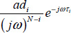
As described previously, HOL(s) has only poles in s = 0. Thus, because in a first step we are only interested in stability, we will apply the simplified Nyquist criterion. HOL(jω) is composed of N terms such as
Hi(jω) is the sum of two basic elements
- 1)
 with modulus
  and polar angle
 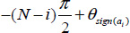 . Its graph is a ray centered at the origin and characterized by its polar angle.
 - 2)
 with modulus
  and polar angle
  .
.
For ω = 0, its graph belongs to a ray similar to the previous one; on the contrary, for ω → +∞, its graph is a spiral centered at the origin caused by the rotation of the polar angle due to the time delay.
The graph of Hi(jω) is the composition of these two basic elements. It depends on:
- – the respective signs of ai and adi;
- – the absolute values of ai and adi.
Specifically, if |ai| ≫ |adi|, then the graph is close to that of the first term, and if |ai| ≪ |adi|, then the graph is close to that of the second term.
Finally, the graph of HOL(jω) results from the composition of the N elementary graphs.
REMARK 4.– The interest of this analysis of elementary graphs is to investigate the influence of each component Hi(jω) in order to formulate analytical conclusions.
If the only objective is to test the stability of a time-delayed ODE, then it is only necessary to compute numerically HOL(jω) for an appropriate choice of frequency values ranging from ω = 0 to ω → +∞ and to plot the corresponding curve: thus, this method can be applied easily to a large variety of systems.
6.5.4. Application to an example
Our objective is to demonstrate that this method gives the same analytical results as other approaches with a reference example.
Consider the well-known system [NIC 97, RIC 03]:
where a0 = a and ad0 = b.
Stability conditions are presented using a {a, b} plane representation. In this example
with
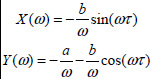
At the limit of stability, the H OL (jω) Nyquist diagram goes through the critical point and X(ω) = –1; Y(ω) = 0.
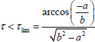
The condition Y(ω) = 0 imposes ![]() which has a solution only if
which has a solution only if ![]() .
.
This condition defines two straight lines in the {a,b} plane: a = b and a = –b which define eight sectors numbered 1–8 (see Figure 6.18).

Figure 6.18. Definition of sectors in the {a, b} plane
It is necessary to determine H OL(jω) in each sector in order to analyze stability. We will investigate only the stability in sectors 1 and 2 in order to demonstrate the application the method, and present the global results for the {a,b} plane.
Sector 1 is characterized by b > a. Thus, the graph of H OL(jω) is close to that of ![]() .
.
Equation [6.71] has a solution:
For this value of ω, the system is stable if: X(ω) > –1 when Y(ω) = 0.
Simple calculations give
Thus, the system is conditionally stable.
Sector 2 is characterized by b < a. Thus, the graph of H OL(jω) is close to that of ![]() .
.
The condition Y(ω) = 0 can be fulfilled only when X(ω) → 0 (with ω → +∞).
Thus, it means that the Nyquist diagram of H OL(jω)is always situated on the “right side” of the critical point: the system is always stable, independently of the value of the time delay τ.
Applying this method to each sector, we finally obtain the results expressed in Figure 6.19.

Figure 6.19. Stability regions in the {a, b} plane
Of course, this stability result is identical to the results presented in [NIC 97, RIC 03].
6.6. Stability analysis of FDEs with time delays
6.6.1. Definitions
We are interested in linear FDEs with time delays whose transfer function ![]() is a generalization of the integer order case:
is a generalization of the integer order case:
with
and where the internal derivative orders ni correspond to the definition [6.3]. Then, the open-loop transfer function H OL(s) is expressed by
6.6.2. Stability
As in the integer order case, we will consider the position of the Nyquist diagram H OL(jω) with respect to the critical point.
H OL (jω) is composed of N terms such as
Hi(jω) is the sum of two basic elements:
- 1)
 with modulus
  and polar angle
  . Its graph is a ray centered at the origin and characterized by its polar angle;
 - 2)
 with modulus
  and polar angle
  .
.
For ω = 0, its graph belongs to a ray similar to the previous one; on the contrary, for ω → +∞, its graph is a spiral centered at the origin.
The graph of H(jω) is the composition of these elementary graphs, as in the integer order case.
Finally, the graph of H OL(jω) results from the composition of the N elementary graphs: the system is stable if the Nyquist diagram lays on the “right side” of the critical point.
6.6.3. Application to an example
In order to test this method, we will apply it to a system where the stability condition is already known, thanks to another approach. This example is the following, given by [HWA 06]. Its characteristic polynomial A(s) is
This example deals with the commensurate order hypothesis: then, n1 = n2 = 0,5. Moreover, the time delay is also fractional of the form ![]() . However, this non-usual form is not an obstacle to the use of the method (with the values a0 = a1 = 1).
. However, this non-usual form is not an obstacle to the use of the method (with the values a0 = a1 = 1).
Then
which can be expressed as
with
and
The graph of H2 (jω) lies between two asymptotes:
- – a ray centered at the origin, with polar angle equal to
 , corresponding to ω =0;
 - – a ray centered at the origin, with polar angle equal to
 , corresponding to ω → +∞.
The transfer function is characterized by: H1(jω) = with ![]() and
and ![]() .
.
⍴1 decreases from K to 0, whereas θ1 varies from 0 to –∞, when ω varies from 0 to +∞.
The graph of H1(jω) is a spiral centered at the origin, and the Nyquist diagram of HOL(jω) is the composition of the two previous graphs.
Stability is conditional, according to the value of K. Let us determine the value of K (Klim) corresponding to the situation where the Nyquist diagram goes through the critical point.
Therefore, HOL (jω) = ⍴ejθ with ⍴ = 1 and θ = – π.
![]() is a solution of the equation
is a solution of the equation
whereas K is obtained from the condition ⍴ = 1 (with the previous value of ![]() ).
).
For τ = 1s, we obtain ![]() and Klim = 21,51 (of course, the same value as provided by [HWA 06]).
and Klim = 21,51 (of course, the same value as provided by [HWA 06]).
The diagrams corresponding to K = {5;10;15;Klim} are plotted in the Nyquist plane (see Figure 6.20).
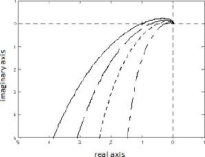
Figure 6.20. Nyquist’s diagram for different values of K
We can verify that the stability is ensured for K < 21,51 . Moreover, the distance between HOL (jω) and the critical point makes it possible to quantify the stability degree of this time-delayed FDE.