
7
Fractional Energy
7.1. Introduction
The application of Lyapunov’s method is based on the definition of a positive quadratic function, related to energy [LYA 07, LAS 61, KRA 63, NAS 68].
For linear integer order systems, the choice of this function V(t) is an elementary problem. Because V(t) should be a quadratic function of state x(t) (or ![]() ), the choice V(t) = x2(t) or as a generalization
), the choice V(t) = x2(t) or as a generalization ![]() with P > 0 is straightforward [KAI 80, KHA 96].
with P > 0 is straightforward [KAI 80, KHA 96].
Many researchers have used the same definition of V(t) in the fractional order case [AGU 14]. Unfortunately, x(t) (or ![]() ) is only a pseudo-state vector and V(t) = x2(t) is a positive semi-definite function which cannot be used as a Lyapunov function, as will be demonstrated using an elementary example.
) is only a pseudo-state vector and V(t) = x2(t) is a positive semi-definite function which cannot be used as a Lyapunov function, as will be demonstrated using an elementary example.
In fact, the true state of the fractional integrator is the distributed variable z(ω,t) (Ẕ(ω,t) for a multidimensional system). Therefore, V(t) has to be a quadratic function based on z(ω,t).
Thus, the definition of V(t) is no longer an elementary problem as in the integer order case. We previously a priori defined V(t) as
in the monovariable case [TRI 11b]. Is it possible to validate this choice using an energetic interpretation?
This is a main objective of this chapter. It will be demonstrated that equation [7.1] corresponds within a factor to the energy stored in a fractional integrator.
In order to prove this definition of fractional energy, we will use an electrical analog [HAR 15a] which will also be used to define the associated dissipation of energy, which is a specific feature of fractional systems. Moreover, we will raise a fundamental question: is fractional energy a simple mathematical function or a true energy?
Comparisons between the energies stored in the infinite length RC line and the fractional integrator (as well as between integer and fractional order integrators) will make it possible to provide a conclusive response to this important question.
Finally, the energy stored in an elementary fractional differential system will be defined using both distributed representations, i.e. the closed-loop and open-loop forms. More precisely, it will be proved that this energy is expressed as the energy stored in the associated integrator in the closed-loop form, whereas a specific expression will be established for the open-loop form. These two equivalent expressions of fractional energy will be used in the stability analysis of commensurate order fractional systems.
7.2. Pseudo-energy stored in a fractional integrator
The objective of this section is to demonstrate that the function x2 (t) does not correspond to an energy in the case of the fractional integrator.
We will use the signal i(t) of Figure 7.1 as an input of the fractional integrator ![]() .
.

Figure 7.1. Fractional integrator input. For a color version of the figures in this chapter see www.iste.co.uk/trigeassou/analysis2.zip
This signal i(t) is realized as the sum of delayed step signals as shown in Figure 7.2.
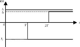
Figure 7.2. Realization of the input
Therefore, the signal i(t) is defined as

This signal i(t) is applied to the input of the fractional integrator (see Figure 7.3).
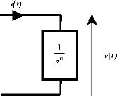
Figure 7.3. Fractional integrator
Thus, the input is i(t), and the output is v(t) such as
Note that the analogy with a fractional capacitor will be justified in section 7.3.
Thus, we can define v(t) at different instants t:
- – for

therefore ![]() and
and ![]()
- – for

We want v(2T) = 0.
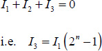
Therefore

which implies
- – finally, for 2T ≤ t, we want i(t) = 0
therefore
Consequently:
We have determined v(t) considering that the fractional integrator is submitted to the different excitations i1 (t), i2 (t) and i3 (t) for t ≥ 2T. However, we can also interpret v(t) for t ≥ 2T as the result of the excitation i(t) of Figure 7.1, i.e. the output v(t) represents the free response of ![]() for t ≥ 2T, starting from v(2T) = 0 with the initial state z(ω,2T), because i(t) = 0 for t ≥ 2T.
for t ≥ 2T, starting from v(2T) = 0 with the initial state z(ω,2T), because i(t) = 0 for t ≥ 2T.
Of course, we have already demonstrated that the free response does not depend on the pseudo-state v(2T) = 0, but on the internal state z(ω,2T), which is not equal to zero regardless of the frequency ω.
For an integer order integrator, the energy E(t) is expressed as ![]() . Therefore, we can define a pseudo-energy
. Therefore, we can define a pseudo-energy ![]() for the fractional integrator, defined similarly as
for the fractional integrator, defined similarly as
In Figure 7.4, we present the response v(t) and the pseudo-energy ![]() for n = 0.5.
for n = 0.5.

Figure 7.4. Pseudo-energy of the fractional integrator
Of course, we note that ![]() since v(2T) = 0 . Furthermore, there is an increase of
since v(2T) = 0 . Furthermore, there is an increase of ![]() for t ≥2T. This increase of
for t ≥2T. This increase of ![]() is not coherent with the initial value of
is not coherent with the initial value of ![]() at t = 2 T. Thus, we can conclude that
at t = 2 T. Thus, we can conclude that ![]() does not correspond to the true energy stored in
does not correspond to the true energy stored in ![]() .
.
We know from Chapter 6 of Volume 1 that x(t) does not represent the true state of the system. Thus, it will be necessary to express the true energy E(t) with the distributed variable z(ω,t) instead of x(t).
REMARK 1.– We can formulate a theoretical interpretation to the physical inconsistency of pseudo-energy ![]() .
.
As
the function
is equal to zero for any combination of the components of z(ω,t) such that ![]() .
.
It is what occurs at t = 2T thanks to the special input i(t) of Figure 7.1. Because there is an infinity of possibilities to obtain v(t) = 0 for any value of t, this means that the pseudo-energy ![]() is a positive semi-definite quadratic form; thus, it cannot represent an energy nor be used as a Lyapunov function in the fractional order case [NAS 68, KHA 96].
is a positive semi-definite quadratic form; thus, it cannot represent an energy nor be used as a Lyapunov function in the fractional order case [NAS 68, KHA 96].
Consequently, it is necessary to define a new expression for the energy, based on the distributed variable z(ω,t).
7.3. Energy stored and dissipated in a fractional integrator
7.3.1. Introduction
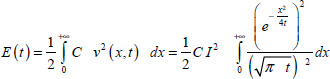
An elementary energy can be defined as
in the frequency band dω, and the global energy E(t) can be defined as the weighted integral of e(ω,t), i.e.
This is the definition of the Lyapunov function V(t) = E(t) which has been successfully used in several papers dealing with stability [TRI 11b, TRI 13b, TRI 13c, TRI 14].
Nevertheless, this definition can be considered as arbitrary because we can ask some questions:
- – Is the choice
 dω realistic?
 - – Is the weighting function μn(ω) necessary?
- – Does V(t) possess the same physical properties as the energy stored in a capacitor, i.e. in the integer order integrator?
In order to provide satisfying answers to these questions, we will interpret the fractional integrator as a frequency distributed network {R(ω),C(ω)} fed by a current i(t) and providing a voltage v(t), according to Figure 7.5.
7.3.2. Electrical distributed network
The structure of the distributed network cannot be chosen arbitrarily, because it has to fit perfectly to the distributed equations of integrator ![]() .
.
Therefore, consider an infinity of elementary parallel {R(ω),C(ω)} cells, connected in series, according to the diagram in Figure 7.5 [HAR 15a, HAR 15b].
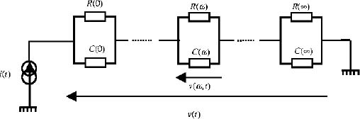
Figure 7.5. Distributed electrical network
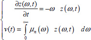
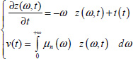
Here, C(ω) and R(ω) are resistor and capacitor densities at frequency ω. In this analogy, i(t) is the input and v(t) is the output. i(t) and v(t) have to verify the distributed model of the integrator ![]() , with the internal variable z (ω,t) :
, with the internal variable z (ω,t) :

According to the network structure, v(t) is the sum of the elementary voltages v(ω,t), therefore
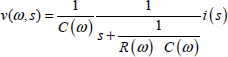
For the elementary cell, we can write
where ZRC(ω,s) is the complex impedance:
Therefore

The Laplace transform of equation [7.10] gives
and
According to [7.11]
Therefore, equations [7.16] and [7.17] are identical if
Then, using [7.14] and [7.15], we obtain

The equality [7.19] is satisfied if
and
7.3.3. Stored energy
The interest of the previous analogy is to allow the calculation of the energy stored in the fractional integrator thanks to the energy stored in the elementary capacitors C(ω).
Let e(ω,t) be the energy density stored in the elementary cell:
As µn(ω) z(ω, t) = v(ω, t) (see [7.18]), we can write
The elementary energy de(ω,t) stored in the band dω is expressed as
Thus, the total energy E(t) stored in the integrator is
This expression of the energy corresponds within a factor to the a priori definition [7.1].
This electrical analogy proves that E(t) has to be weighted by µn (ω). Note that the expression ![]() would be independent of the order n, which obviously would exhibit some inconsistency!
would be independent of the order n, which obviously would exhibit some inconsistency!
7.3.4. Power dissipated in the fractional integrator
The electrical analogy also reveals that an electrical power is dissipated in the distributed resistors R(ω).
Using equations [7.20] and [7.21], we obtain
The power density dissipated in R(ω) is expressed as
As v(ω,t) = µn(ω) z(ω, t) [7.18], we obtain
therefore
where dp(ω,t) is the Joule power dissipated in the frequency band dω.
Finally, the total power P(t) dissipated in ![]() is defined as
is defined as
We note that the energy storage E(t) in the fractional integrator is necessarily associated with a power loss P(t): this is an essential feature of the fractional integrator.
We will demonstrate in the chapters devoted to Lyapunov stability (Chapters 8–10) that this power loss increases the damping of system dynamics, i.e. it improves the natural stability of fractional order systems.
7.3.5. Energy storage
7.3.5.1. Introduction
The infinite length {R,C} line has already been studied in Chapter 6 of Volume 1. It was demonstrated that the { R,C} line is equivalent to a fractional integrator with the order n = 0.5.
Basically, we can calculate the stored energy in this line thanks to physics. Furthermore, equation [7.25] provides the value of the energy stored in the equivalent fractional integrator. The comparison of these two values will allow the validation of equation [7.25].
The infinite length {R,C} line is composed of an infinity of elementary cells {Rdx,Cdx}, according to the diagram in Figure 7.6.
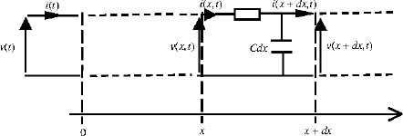
Figure 7.6. Infinite length RC line
R and C are densities per unit length, such as:
Let us recall that the distributed variables v(x,t) and i(x,t) verify the diffusion equation:

with the boundary condition at x = 0:
We have proved that the {R,C} line is equivalent to the fractional integrator (see Chapter 6 of Volume 1):
7.3.5.2. Energy stored in the RC line
Consider a Dirac excitation of the { R,C} line
Therefore
and
As (see Chapter 6 of Volume 1)
and using R = 1 and C = 1 as a simplification, we obtain
Therefore
For each elementary cell, the stored energy density is expressed as
Therefore, for the total stored energy:
and finally [HAR 15a]
We can also calculate E(t) with equation [7.25].
It is necessary to calculate z(ω,t), which is the solution of the differential equation [7.10]. Therefore
Then
As (Appendix A.1, Chapter 1 of Volume 1)
we obtain
Finally, with n = 0.5
As equations [7.43] and [7.48] are identical, this equality proves that the energy stored in a fractional integrator is equal to the energy stored in an infinite length {R,C} line. Obviously, this equality validates equation [7.25].
7.3.6. Integer order and fractional order integrators
7.3.6.1. Integer order integrator
The integer order integrator is characterized by the equation
An operational amplifier realization of this integrator corresponds to the diagram in Figure 7.7 [AUV 80, CHA 82].

Figure 7.7. Integer order integrator
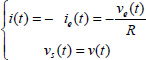
In this system

Basically, this electronic system corresponds to the charge of a capacitor C with a current source i(t), according to the diagram in Figure 7.8.
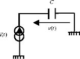
Figure 7.8. Equivalent electrical circuit
Therefore
This equation corresponds to [7.49] with C = 1.
REMARK 2.– We can note that capacitor C replaces the electrical network {R(ω),C(ω)} of Figure 7.5, i.e. we can propose a realization of the fractional integrator using an operational amplifier and the { R(ω),C(ω)} electrical network, according to the diagram in Figure 7.9.
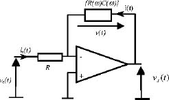
Figure 7.9. Fractional order integrator
The fractional integrator is characterized by the electrical equations:
i.e.
7.3.6.2. Energy stored in the integer order integrator with a step input excitation
Let us consider a step input excitation of the integer order integrator
Therefore, equation [7.51] provides
i.e.
Then, with v(0) = 0, we obtain ![]() and
and
where E1(t) is the energy stored for n = 1.
Then, with C = 1
7.3.6.3. Energy stored in the fractional order integrator with a step input excitation
Consider the step input excitation i(t) = IH(t).
Then, z(ω,t) is the solution of the differential equation:
Therefore
and
Thus
This integral is calculated using the integration by parts technique.
Consider
Let us define
and
Then
As
we obtain
Finally, as Γ(α+1) = α Γ(α) and ![]() (see Chapter 1 of Volume 1), we obtain
(see Chapter 1 of Volume 1), we obtain
Let us recall that ![]() , for the integer order integrator.
, for the integer order integrator.
Thus, if n → 1 in equation [7.69], we obtain:
This result means that the energy stored in the fractional integrator corresponds to the energy stored in the integer order integrator, which can be interpreted as a particular case of the fractional integrator.
Moreover, equation [7.69] demonstrates that the energy stored in ![]() is finite regardless of the finite value t, as in the integer order case.
is finite regardless of the finite value t, as in the integer order case.
This stored energy, or fractional energy, is characterized by the same physical features as in the integer order case.
However, there is an essential difference: energy dissipation is necessarily associated with energy storage in the fractional order case, in contrast to the integer order case.
7.3.6.4. Numerical simulation of stored energy
The fractional integrator is simulated thanks to a frequency discretization (see Chapter 2 of Volume 1):
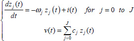
After discretization, equation [7.25] becomes
Our objective is to verify that whether this equation can provide a correct approximation of the fractional energy.
Thus, we simulate the response of the integrator with a step input excitation i(t) = IH(t), where the exact value of En(t) is known:
Then, we can compare En (t) to the numerical approximation [7.72], performed with the simulation parameters ωb =10–3rd/s, ωh=103rd/s, J = 20, I = 1 and n = 0.5.
Consequently, consider the graphs in Figure 7.10.

Figure 7.10. Theoretical and simulated energies
We note the perfect fit between the two curves.
Then, we can compute the energy stored in ![]() with the excitation i(t) of Figure 7.1, with the same simulation parameters (see the graph in Figure 7.11).
with the excitation i(t) of Figure 7.1, with the same simulation parameters (see the graph in Figure 7.11).
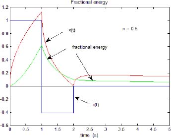
Figure 7.11. Fractional energy
It is now obvious that E(2T) is not equal to zero, in contrast to pseudo-energy ![]() .
.
Moreover, this initial value E(2T) explains the decrease of E(t) since t = 2T.
7.3.7. Characterization of fractional energy and its dissipation
7.3.7.1. Introduction
Equations [7.25] and [7.30] define respectively energy storage E(t) and power dissipation P(t) in the fractional integrator. Comparison with the integer order integrator has exhibited some physical features of fractional energy. However, we can still raise some questions on the distribution of this energy between the different modes ω and also on the relation between energy storage and its dissipation.
7.3.7.2. Modal distribution of energy storage
What happens to En(t) with a step input excitation when t → +∞?
Of course, ![]() as well as
as well as ![]() .
.
However, what is the distribution of stored energy between the different modes as t → +∞?
Let us recall [7.62]: 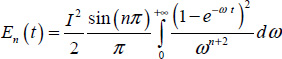 .
.
Moreover, we can note that ![]() .
.
Therefore, let us define
It is straightforward to verify that
as predicted by equation [7.73].
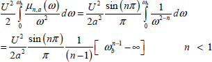
However, we can note that En, ωb (∞) represents the energy stored in the modes ω ranging from ω = ωb to ω → ∞ as t → ∞.
Equation [7.74] demonstrates that this energy is finite. Moreover, if ωb is increased, En, ωb (∞) decreases, i.e. the high frequency modes provide a negligible contribution to the stored energy.
In fact, En, ωb (∞) → ∞ as predicted by [7.73], only thanks to the mode ωb = 0. Obviously, it is the same mechanism as in the integer order case where the only mode is ω = 0 . This is a fundamental property of the fractional integrator.
7.3.7.3. Energy dissipation
Let us recall that power loss P(t) is defined by equation [7.30]:
Let Ed (t) be the energy dissipated in the fractional integrator. It is defined by
What is the value of Ed (t) with the step input excitation?
We know that ![]() , therefore
, therefore
We can calculate this integral using the integration by parts technique. Thus, we obtain
It is straightforward to verify that P(t) = 0 for n = 1, i.e. there is no power loss in the integer order integrator.
Then, using [7.77], we can calculate Ed (t).
Thus, we obtain
7.3.7.4. Energy balance in the fractional integrator
Let EG (t) be the energy provided by the generator.
Therefore,
Using equations [7.73] and [7.80], we obtain
If n → 1, then Ed(t) → 0; therefore, ![]() , i.e. all the stored energy is equal to the energy provided by the generator, since 2 power loss is equal to zero.
, i.e. all the stored energy is equal to the energy provided by the generator, since 2 power loss is equal to zero.
On the contrary, if n → 0 En (t) → 0, and EG(t) → I2t, i.e. if n → 0, the fractional integrator does not store energy, and all the energy provided by the generator is dissipated.
7.3.7.5. Fractional integrator auto discharge
After a charge phase with a step input excitation (i(t) = IH(t)), assume that i(t) = 0 for t ≥ T.
Let us recall the behavior of the integer order integrator:
Let us change the time origin at T (for a simplification objective). Then, t’ replaces t – T. At t’ = 0 (t = T), we have v(0) = v(T) since i(t’) = 0 for t’ ≥ 0, then ![]() , so v(t’) = v(0) = cte.
, so v(t’) = v(0) = cte.
Similarly, ![]() .
.
It is well known that the integer order integrator stores energy from 0 to T, and holds it for t ≥ T.
The behavior is completely different in the fractional order case.
With the new time origin, and using t for t’, we can write (for t ≥ T):
Thus, we obtain
where z(ω,0) = z(ω,T).
and
Thus, ∀ ω, z(ω,t) → 0 as t → ∞ with a decrease speed depending on the mode ω.
For the energy, we can write
Since e–2ωt → 0 as t → ∞, energy En(t) is decreasing. Is it possible to characterize this decrease?
At t = 0, it is obvious that
The derivative ![]() characterizes the decrease
characterizes the decrease
As 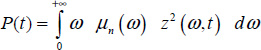 , we obtain
This means that the energy stored previously in the integrator is spontaneously dissipated in resistors R(ω); this is an auto discharge phase.
We can also write ![]() , i.e. the energy stored during the phase charge (when i(t) = IH(t)) is completely dissipated inside the integrator when i(t) = 0, i.e. during the discharge phase or auto dissipation phase.
, i.e. the energy stored during the phase charge (when i(t) = IH(t)) is completely dissipated inside the integrator when i(t) = 0, i.e. during the discharge phase or auto dissipation phase.
We can conclude that the fractional integrator is unable to hold the energy stored during the charge phase.
This is the main difference between the integer and the fractional order integrators: surprisingly, the fractional integrator (or equivalently the fractional capacitor) is not an energy storage device.
7.3.8. Fractional energy invariance
7.3.8.1. State-space models of the fractional integrator
The state space model of the fractional integrator is provided by the inverse Laplace transform of ![]() (see Chapter 6 of Volume 1). In fact, this technique only provides the impulse response of the integrator:
(see Chapter 6 of Volume 1). In fact, this technique only provides the impulse response of the integrator:
which can be interpreted as a state-space model.
Moreover, according to the system theory [KAI 80, ZAD 08], the state space model of a system with input i(t) and v(t) is not unique. Thus, we can define an infinity of state space models, corresponding to the same input/output behavior.
For ![]() , two models can be privileged:
, two models can be privileged:
Model no. 1
Model no. 2
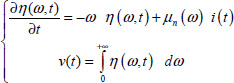
The difference between these two models relies on their distributed variables z(ω,t) and η(ω,t), and also on the position of the weighting function: on the output or on the input.
We are interested in the definition of the energy of each model, in order to verify the invariance principle [JOO 86].
7.3.8.2. Stored energy of the two models
The stored energy of model no. 1 has been expressed using the distributed network analogy (see sections 7.3.2 and 7.3.3).
Thus we have already defined [7.25],  .
.
For model no. 2, we use the same analogy (see Figure 7.5). The elementary cell is characterized by the equation
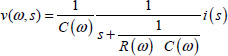
As
we obtain
as
equality [7.95] implies that:
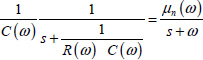
Therefore, this equality is verified if
For the elementary cell
Thus, the total energy Eη(t) is defined as
7.3.8.3. Invariance of energy
First, the expressions of Ez(t) and Eη(t) seem different.
In fact, we can express η (ω,t) as a function of z(ω, t).
Note that ![]() and
and ![]() .
.
Therefore
thus Eη(t) becomes

i.e.
We would get the same result with any other model; hence, we have revisited a fundamental principle of energy [JOO 86].
Energy is an invariant of the fractional integrator. This principle can be generalized to any fractional system, i.e. energy is independent of the modeling of this system.
7.4. Closed-loop and open-loop fractional energies
7.4.1. Introduction
Energy is a fundamental topic in system stability analysis based on the Lyapunov method. In the integer order case, the energy of the elementary system ![]() is expressed as
is expressed as ![]() , corresponding to the energy stored in the associated integrator.
, corresponding to the energy stored in the associated integrator.
This principle can be generalized directly to the fractional elementary system ![]() thanks to the distributed variable z(ω,t). The specificity of the fractional order case is due to the availability of two distributed models, a classical one in a closed-loop form with the variable z(ω,t) and another one in an open-loop form with the variable ξ(ω,t) (see Chapter 7 of Volume 1). Consequently, it will be necessary to express its energy with ξ(ω,t).
thanks to the distributed variable z(ω,t). The specificity of the fractional order case is due to the availability of two distributed models, a classical one in a closed-loop form with the variable z(ω,t) and another one in an open-loop form with the variable ξ(ω,t) (see Chapter 7 of Volume 1). Consequently, it will be necessary to express its energy with ξ(ω,t).
Finally, the interest of these equivalent definitions of system energy will be illustrated to express the initialization energy of the Caputo derivative.
7.4.2. Energy of the closed-loop model
Let us recall the definition of the energy of the elementary integer order system ![]() which corresponds to the ODE
which corresponds to the ODE
This model corresponds to the closed-loop diagram in Figure 7.12.

Figure 7.12. Closed-loop ODE model
x(t) is the output (and the state variable) of integrator ![]() . Its input is v(t):
. Its input is v(t):
The integrator ![]() is the unique storage device of this closed-loop system. The energy E1(t) of the ODE corresponds to the energy stored in the integrator, characterized by the state variable x(t).
is the unique storage device of this closed-loop system. The energy E1(t) of the ODE corresponds to the energy stored in the integrator, characterized by the state variable x(t).
Thus
Usually, this expression is simplified, i.e. this energy is defined as x2 (t), and it is improperly said that x2(t) is the energy of state variable x(t).
In fact, it is necessary to say that E1(t) is the energy stored in the integrator ![]() associated with the modeling of the ODE.
associated with the modeling of the ODE.
Then, consider the fractional order case and the elementary model ![]() corresponding to the FDE:
corresponding to the FDE:
This model corresponds to the closed-loop diagram in Figure 7.12, where the integrator ![]() is replaced by
is replaced by ![]() .
.
Therefore, x(t) is the output of the fractional integrator characterized by the distributed internal variable z(ω,t). The input of the integrator is v(t):
Consequently, the distributed model of the elementary FDE is:

The distributed state variable z(ω,t) of ![]() is also the state variable of the FDE, whereas x(t) is only a pseudo-state variable (see Chapter 6 of Volume 1). The only energy storage device is the integrator
is also the state variable of the FDE, whereas x(t) is only a pseudo-state variable (see Chapter 6 of Volume 1). The only energy storage device is the integrator ![]() associated with the FDE.
associated with the FDE.
Thus, the stored energy of the FDE is defined as:
REMARK 3.– Note that it would have been possible to use model no. 2 of section 7.3.8, characterized by the variable η(ω,t). The energy of the FDE would have been defined as:
However, recall that according to the invariance principle, we have Eη(t) = Ez(t).
7.4.3. Energy of the open-loop model
The open-loop distributed model of the elementary system ![]() is provided by the inverse Laplace transform (see Chapter 7 of Volume 1).
is provided by the inverse Laplace transform (see Chapter 7 of Volume 1).
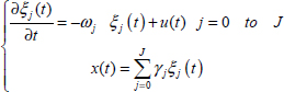
Thus, we can write
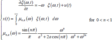
In this state space model, the previous distributed variable z(ω,t) has been replaced by ξ(ω,t). This new variable does not refer to any integrator ![]() ; thus, it is necessary to avoid the confusion between ξ(ω,t) and z(ω,t).
; thus, it is necessary to avoid the confusion between ξ(ω,t) and z(ω,t).
Although the distributed differential equations share the same structure, note that they fundamentally differ by their excitation: u(t) – ax(t) for the closed-loop form and u(t) for the open-loop form.
In order to express the energy stored by the open-loop model, we use the same electrical network analogy as with the fractional integrator, with i(t) which is the input corresponding to u(t), and v(t) to x(t) (see Figure 7.5).
For the elementary cell:
as
we obtain
As
we obtain the equality

The validation of this equality requires that
Moreover, the energy stored in all the distributed capacitors is defined as
According to equations [6.115] and [6.118], we finally obtain
Of course, because the closed-loop model and the open-loop one correspond to the same system ![]() , the invariance principle imposes En,ξ(t) = En,z(t).
, the invariance principle imposes En,ξ(t) = En,z(t).
7.4.4. Stored energies with a step input excitation
7.4.4.1. Energy stored in the closed-loop model
Using the Laplace transform, we can write, with an initial condition equal to zero (z(ω, 0) = 0 ∀ω)
Therefore
Thus
and
As u(t) = UH (t), i.e. ![]() , we obtain
, we obtain
Thus, we can calculate z(ω, ∞).
We know that
Therefore, according to [7.125]
and
Furthermore
Thus, x(∞) has a finite value, whereas z(0, ∞), the modal component of x(t) at ω = 0, has an infinite value.
As ![]() and z(ω, ∞) = 0 ∀ω ≠ 0, we obtain
and z(ω, ∞) = 0 ∀ω ≠ 0, we obtain
This means that the high frequency modes of z(ω, t) have a limited contribution to global stored energy, even equal to zero as t → ∞.
Thus, intuitively, we can say that En,z(∞) → ∞ because z(0, ∞) and µn(0) → ∞.
Using the open-loop model and the invariance principle, we can provide a more convincing proof to this result.
REMARK 4.– The previous result also means that the energy of the closed-loop model is mostly stored in the mode ω = 0.
7.4.4.2. Energy stored in the open-loop model
Using the Laplace transform, we can write with an initial condition equal to zero (ξ(ω, 0) = 0 ∀ω).
In contrast to the closed-loop model, ξ(ω,t) exhibits a simple analytical expression:
Then
Note that 1– e–ωt → 1 as t → ∞
Therefore
with
Therefore, as ω → ∞.
thus
On the contrary, as ω → 0
Let ωb be a frequency close to 0 .
Therefore, we can write
The second integral provides a finite contribution to the stored energy: it represents the contribution of higher frequency modes.
Furthermore, for the first integral, we can write:
Thus, En,ξ(∞) → ∞ as t → ∞.
REMARK 5.–
Thus, ξ(0,t) = Ut and ![]() .
.
ξ(0,t) corresponds to the integer order behavior, and it explains why the energy stored in the open-loop model tends to infinity.
7.4.4.3. Numerical simulation of stored energy
Let us recall that the frequency discretized model of the closed-loop form is

and the frequency discretized model of the open-loop form is
Thus, the stored energies Ez(t) and Eξ(t) are expressed by the discrete sums:

Numerical simulation of x(t), Ez(t) and Eξ(t) is performed for U = 1 with the following parameters: ωb=10–3rad/s, ωh = 10+3 rad/s, J = 20, a = 1 and Te =10–3 s.
The graphs of x(t), Ez(t) and Eξ(t) are presented in Figure 7.13.
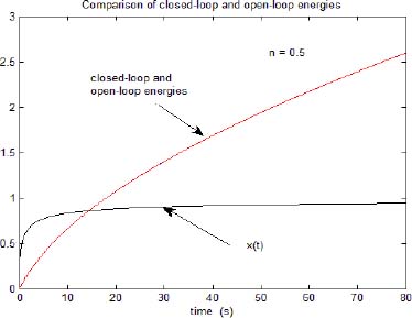
Figure 7.13. Closed-loop and open-loop energies
As theoretically expected, x(t) tends asymptotically to x(∞) = 1. Note that the graphs of Ez(t) and Eξ(t) fit perfectly, which is the experimental validation of the invariance principle: Ez(t) = Eξ(t).
Moreover, we verify that stored energy tends asymptotically to infinity, whereas x(t) tends to a finite value as t → ∞.
REMARK 6.– Consider the integer order system ![]() .
.
Its response to the step input U H(t) is ![]() with
with ![]() , as demonstrated previously.
, as demonstrated previously.
Its stored energy is defined as ![]() . As
. As ![]() , we obtain
, we obtain ![]() .
.
Thus, there is a fundamental difference between the energy stored in a fractional order system and in an integer order system.
7.4.4.4. Application: initialization energy of the Caputo derivative
Consider the elementary FDE:
At t = 0 , the usual initial condition of the Caputo derivative is defined as x(0) (see Chapters 3 and 8 of Volume 1).
Let us recall that this derivative is given by:
which corresponds to the distributed system (see Chapter 8 of Volume 1):
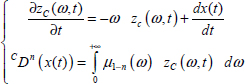
Let us recall that zC (ω,t) is the distributed internal variable of integrator ![]() , which must not be mistaken with the distributed variable z(ω,t) of the closed-loop model.
, which must not be mistaken with the distributed variable z(ω,t) of the closed-loop model.
Let zC(ω, 0) and x(0) be the values at t = 0.
Let us recall (see Chapter 8 of Volume 1) that
and
The only way that x(0) can be the initial condition of the Caputo derivative is that zC (ω,0) = 0 ∀ ω.
According to [7.146], this condition implies that ![]() for t < 0, since t = –∞, i.e. x(t) = cte since t = – ∞.
for t < 0, since t = –∞, i.e. x(t) = cte since t = – ∞.
Consider system [7.144] and apply a step input U H(t) since t = –∞.
Thus, using the results of section 7.4.4, we obtain ![]() with
with
This situation corresponds to x(t) = cte since t = –∞, or ![]() for t < 0, i.e. it means that the ideal Caputo’s initial condition is satisfied.
for t < 0, i.e. it means that the ideal Caputo’s initial condition is satisfied.
We demonstrated that the energy stored in the system [7.144], i.e. in its associated integrator ![]() , tends to infinity.
, tends to infinity.
This means that the energy required by the initial condition x(0) = cte since t = –∞, i.e. the energy required by the Caputo’s initial condition has to be infinite.
Consequently, in energy terms, this initial condition x(0) = cte is a physical utopia. This result has also been proved by a more theoretical approach in [HAR 15c].