13
A New Non-monotonic Link Function for Beta Regressions
Beta regression is used to analyze data whose value is within the range (0,1), such as rates, proportions or percentages, and therefore is useful for analyzing the variables that affect them (Ferrari and Cribari-Neto 2004; Simas et al. 2010). This method is based on the beta distribution or its re-parametrizations, proposed by Ferrari and Cribari-Neto (2004) and Cribari-Neto and Souza (2012), to obtain a regression structure on the mean that is easier to analyze and interpret. For the regression for binary data, the literature has debated the problem of incorrect link functions and therefore proposed new links, such as gev (generalized extreme value), while, for the mean of the beta regression, the traditional link functions for binary regressions were used, i.e. logit, probit and complementary log–log. In this chapter, a new inverse link function is proposed for the mean parameter of a beta regression, which has as its particular cases inverse logit, representing a traditional symmetric inverse link function, and gev, proposed for binary data due to its asymmetry. The new inverse link function proposed in this chapter has the advantage that it can also be non-monotonic, unlike those proposed until now. The parameters are estimated maximizing the likelihood function, using a modified version of the genetic algorithm, therefore giving greater importance to traditional link functions than the others. This method is compared with the one proposed by Cribari-Neto and Zeileis (2010), in which the researcher decides a priori the link function, using simulated data, so as to be able to compare which of the two methods is closest to the true values. This method, therefore, is better because it is able to correctly determine the link function with which the data was simulated and to estimate the parameters with less error.
13.1. Introduction
Beta regression is typically used to analyze data whose value is within the range (0,1), such as rates, proportions or percentages, and to study the variables which affect them (Cox 1996; Ferrari and Cribari-Neto 2004; Simas et al. 2010; Cribari-Neto and Queiroz 2014). This statistical method is based on beta distribution or its re-parametrizations, proposed by Ferrari and Cribari-Neto (2004) and by Cribari-Neto and Souza (2012), to obtain a regression structure on the mean which is easier to analyze and interpret. Cox (1996) and Kieschnick and McCullough (2003) were among the first to propose beta regression. They proposed their own version of the generalized linear models (McCullagh and Nelder 1989) for the variables of interest included in the unit interval, exploiting the belonging of the beta distribution to the exponential family, on the basis of the generalized linear model. These link the mean of the variable of interest to a function, called the link function, of exogenous explanatory variables, also called regressors. The inverse of the link function is called the response function. Since the mean of the beta distribution is between 0 and 1, Kieschnick and McCullough (2003) recommend the use of a logit link function, essentially created to be applied to regressions for binary data. In its traditional form, the beta distribution is characterized by the two parameters p and q. Because its mean is a function of the parameters p and q, Kieschnick and McCullough (2003) link them to the explanatory variables through the link function, considering q as a function of the regressors. Ferrari and Cribari-Neto (2004) re-parameterize the beta distribution, which thus becomes characterized by the parameters µ and φ, which are, respectively, the mean and the precision. With this modification, the analysis is simplified, since the mean is directly linked to the explanatory variables through the link function. The parameters of the link function are estimated using the quasi-maximum likelihood (QMLE) method (Cox 1996; Kieschnick and McCullough 2003) or the maximum likelihood method (Ferrari and Cribari-Neto 2004). Beta regression has had a further evolution with the possibility of also linking the precision parameter to explanatory variables through another link function (Smithson and Verkuilen 2006; Simas et al. 2010). Smithson and Verkuilen (2006) use the logarithmic function for the link function of the precision parameter and the logit function for the mean. Simas et al. (2010), instead, propose some functions both for the link function of the precision parameter and for that of the mean. Simas et al. (2010) apply, for the mean, the traditional link functions of binary regressions, i.e. logit, probit and complementary log–log, and, for the precision parameter, the logarithmic function, the square root and equality. The parameters of the two link functions are estimated with the maximum likelihood method. Cribari-Neto and Souza (2012) propose their new parameterization of the beta distribution, where the parameters represent the mean and a measure of dispersion. In their study, the logit function is used for both link functions.
In the literature, the problem of incorrect link functions has been discussed in the context of regressions for binary data (Czado and Santner 1992), and therefore, new and further link functions have been proposed (Aranda-Ordaz 1981; Stukel 1988; Nagler 1994; Wang and Dey 2010; Jiang et al. 2013; Gheno 2018). For the mean of the beta regression, however, until now, researchers have used the link functions used for the binary regressions, i.e. logit, probit and complementary log–log. Since the mean is between (0,1), however, only the functions (0,1) →can be used as link functions. The logit and probit functions are monotonic and symmetric functions, while the complementary log–log approaches slowly 0 and quickly 1. The complementary log–log, also defined as extreme minimal value (Fahrmeir and Tutz 2013), has its complementary version in the log–log, or extreme maximal value (Fahrmeir and Tutz 2013), because it approaches 0 quickly and 1 slowly. Other non-symmetric functions have been proposed for binary data. Some examples of these link functions are gev (generalized extreme value), which has the complementary log–log link function as a special case (Wang and Dey 2010; Calabrese and Osmetti 2013); scobit (Nagler 1994) and Aranda-Ordaz’s link, which has the logit and the complementary log–log as special cases (Aranda-Ordaz 1981). Only Canterle and Bayer (2019) use Aranda-Ordaz’s link for the mean in a beta regression.
In this chapter, a new response function is proposed for the mean parameter of a beta regression, which has as its particular cases the symmetric inverse link function logit and the asymmetric gev. The new response function has the advantage that it can also be non-monotonic, a feature not present in those proposed until now. The parameters are estimated with the maximization of likelihood, made possible by the use of a modified version of the genetic algorithm, to give more relevance to the traditional link functions than the others. This new method is compared with that proposed by Cribari-Neto and Zeileis (2010) using simulated data, in order to compare which of the two methods is closest to the true values. This method is able to correctly determine the link function with which the data are simulated and to estimate the parameters with less error.
13.2. Model
The variable of interest of a beta regression has a beta distribution and therefore takes values between 0 and 1, excluded extremes. However, beta regression can also be used for variables included in an interval (a, b) with the appropriate modifications, i.e. (y-a)/(b-a) (Ferrari and Cribari-Neto 2004; Smithson and Verkuilen 2006). If y, instead, can also assume the values 0 and 1, Smithson and Verkuilen (2006) propose the transformation (y (n - 1) + 0.5)/n, where n represents the sample size.
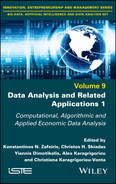
To facilitate the interpretation of the estimated values from the beta regression, Ferrari and Cribari-Neto (2004) propose the following re-parametrization of the beta distribution
where μ represents the mean and is between 0 and 1 excluded, and φ represents the precision parameter and is greater than 0. In this parameterization, the variable y has the mean equal to μ and variance equal to μ (1-μ)/(1 + φ). In the simplest form of beta regression, the mean of the variable of interest is equal to
where xj with j = 1, … , J represent regressors or explanatory variables and g(∙) a function such that g-1(∙): ℜ → (0, 1). The function g(∙) is called the link function (Cribari-Neto and Zeileis 2010) while g-1(∙) is called the response function. In this case, g(∙) represents the link function of the mean. In the most advanced form of beta regression (Smithson and Verkuilen 2006; Simas et al. 2010), indeed, even the precision parameter becomes a linear function of the explanatory variables zk with k = 1, … , K
where h(∙) represents the link function of the precision parameter and is such that h-1(∙):ℜ → (0, ∞) (Cribari-Neto and Zeileis 2010). A sample of sample size n is used to estimate the parameters β and φ of the simpler version or the parameters β and γ of the more complex version. The relative log-likelihood function of the simplest model becomes
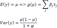
In the simplest version, each observation yi has mean equal to µi and variance equal to µi (1 − µi )/(1 + φ). The parameters are obtained by maximizing the log-likelihood function. The most commonly used link functions for the mean are, respectively, logit, probit and complementary log–log
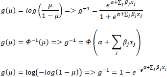
While logit and probit are monotonic and symmetric functions, complementary log–log approaches 0 slowly and 1 quickly. In this chapter, to broaden the possibility of studying the relationship between the mean µi and the explanatory variables xij with j = 1, … J more comprehensively, a new response function called logev is proposed, because it contemplates between its particular cases the inverse link function logit and that gev (Calabrese and Osmetti 2013), until now only applied to regressions for binary variables. The gev link function is
The response function gev becomes with τ → 0 the response function of the complementary log–log and with τ < 0 the response function of Weibull (Calabrese and Osmetti 2013). The logev function is
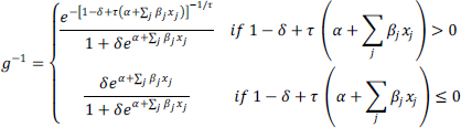
with τ, α, βj ∈ (−∞, +∞) and δ ∈ [0,1]. If δ = 0, the equation becomes the response function gev, if, instead, δ = 1 and τ = −1, the equation becomes the inverse link function logit. The peculiarity of this response function is that the choice of symmetry or asymmetry is not given a priori but by the data. In the response functions proposed until now, this choice is made a priori by the researcher, while in this response function are the data that provide it. As noted by Czado and Santner (1992) in the model of the binomial regression, also for the beta regression, the misspecification of the link function induces the bias of the estimated parameters, and therefore, an a priori choice can eliminate this problem. Another peculiarity of this function is the possibility of being non-monotonic, a feature that has not been considered for a beta regression until now. Non-monotonicity for binary data has only been proposed in the Bayesian field by Gheno (2018).
13.3. Estimation
The parameters of the logev regression cannot be estimated using the maximization of the log likelihood with the derivatives, due to its complexity, and therefore, the use of a modified version of the genetic algorithm presented by Holland is proposed (Holland 1975). Genetic algorithms, based on the concept of evolution, are very often used for optimization problems (Whitley 1994). The algorithm, which is proposed in this chapter, divides the sample into two parts: the train part, which corresponds to 75% of the sample, and the test part, which refers to the remaining 25%. This subdivision is used to analyze the goodness of the estimate (train) and the goodness of the forecast (test). The parameters are estimated applying the genetic algorithm to the likelihood calculated on the train dataset. The MSE (mean square error) is calculated in both datasets (train and test), in order to study both the goodness of the estimate and the goodness of the forecast. Repeating the subdivision of the dataset and the related estimation process 100 times, the parameters that minimize the following two functions are obtained:
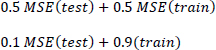
In the first function, equal importance is attributed to goodness of estimate and goodness of forecast; in the second, instead, more importance is given to goodness of estimate. If the estimation of the parameters ![]() determines a known model (logit or gev), the estimate of the parameters
determines a known model (logit or gev), the estimate of the parameters ![]() with j = 1, … J is equal to the estimate obtained from the subdivision v with v = 1, … , 100
with j = 1, … J is equal to the estimate obtained from the subdivision v with v = 1, … , 100
If ![]() , instead, determines an unknown model, the algorithm analyzes the parameters estimated by the following function:
, instead, determines an unknown model, the algorithm analyzes the parameters estimated by the following function:
If these determine a known model, they become the searched estimated parameters. If both functions, instead, determine ![]() of an unknown model, the estimate of the first function is chosen. This procedure is preferred in order to give greater importance to the logit and gev models than a hybrid model. The standard errors of the estimated parameters can be calculated with the bootstrap method.
of an unknown model, the estimate of the first function is chosen. This procedure is preferred in order to give greater importance to the logit and gev models than a hybrid model. The standard errors of the estimated parameters can be calculated with the bootstrap method.
13.4. Comparison
To study the goodness of the method, it is compared with the beta logit regression proposed by Cribari-Neto and Zeileis (2010) (hereinafter also defined as betareg), using simulated data so as to know exactly what the true relationship between the response variable and the explanatory variables is. In the first analysis, 30 datasets of sample size 500 are simulated from a logit model with α = 1 and β = −2. Logev beta regression estimates all datasets, while logit beta regression is able to estimate only 25 datasets. Figure 13.1 shows that in almost 80% of cases, logev chooses the logit model exactly. As simulated data is used, it is possible to analyze which of the two methods is closest to the true value. Only the cases where logev chooses the logit model exactly are considered, and the bias is analyzed (Langner et al. 2003):
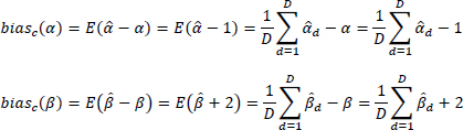
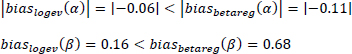
where D is the number of simulated datasets, which are estimated by both methods as logit model and is equal to 19 and c = betareg, logev. If the bias is considered, the intercept and the coefficient β are better estimated by the logev method, because, in both cases, the logev bias is closer to 0 than the betareg bias:
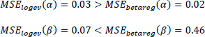
When always considering the cases where logev chooses the logit model exactly, the MSE statistic of the two methods is compared, in order to analyze both the variance and the bias:
where D = 19 and c = betareg, logev. The intercept is better estimated by the betareg method, even if the two MSEs are very close, while logev estimates the coefficient β much better
The two methods are compared with the AIC and BIC criteria. The AIC and BIC are equal to (Qi and Zhang 2001).
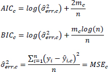
where c = betareg, logev and mc represents the number of parameters and therefore mbetareg = 4, while mlogev = 6. The two AICs are now compared:
If ∆AIC > 0, the best model is logev, and then the condition for choosing the logev is
Now, the BIC is compared:
If ∆BIC > 0, the best model is the one proposed by the logev regression model, and the condition for choosing the logev becomes
Figure 13.2 shows that logev is always better than the logit regression model.
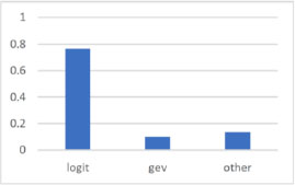
Figure 13.1. Percentage of choice (logit dataset)
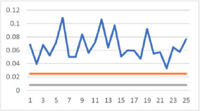
Figure 13.2. Comparison between AIC and BIC, blue = ∆log(MSE), gray = 0.008, orange = 0.024858
In the following three datasets, logev and logit are only compared by analyzing the goodness of the model. Indeed, the estimation of the parameters α and β is not considered, because, as noted by (Czado and Santner 1992), their estimation depends on the type of the used link function. In the first dataset, instead, the estimation of the parameters α and β is compared because logev also chooses the link function logit. In the second analysis, 30 datasets of sample size 500 are simulated from a gev model with α = 1, τ = −4, β = −2. In this case, logev always correctly chooses the gev model (Figure 13.3), but estimates better in only about 60% of cases (Figure 13.4).
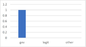
Figure 13.3. Percentage of choice (gev data)
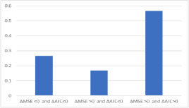
Figure 13.4. Comparison of AIC and of MSE (if ∆MSE > 0, according to MSE the best model is logev)
In the third analysis, 30 datasets of sample size 500 are simulated from a gev model with α = 1, τ = 1, β = −2. In this case, logev almost always correctly chooses the gev model (Figure 13.5) and estimates better in about 90% of cases (Figure 13.6).
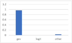
Figure 13.5. Percentage of choice (gev data)
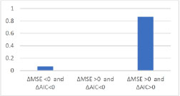
Figure 13.6. Comparison of AIC and of MSE (if ∆MSE > 0, according to MSE the best model is logev)
In the fourth analysis, 30 datasets of sample size 500 are simulated from a non-monotonic model:
The logev method is always able to estimate the model, while logit beta regression is only able to estimate the model 28 times. In this case, logev chooses the correct model in almost 75% of cases (Figure 13.7) and estimates better in about 99% of cases (Figure 13.8).
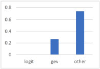
Figure 13.7. Percentage of choice (non-monotonic data)
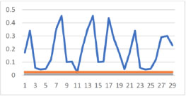
Figure 13.8. Comparison between AIC and BIC, blue = ∆log(MSE), gray = 0.008 and orange = 0.024858
13.5. Conclusion
The study of the link functions in the case of beta regression has, until now, been poorly developed, and therefore, in this chapter, a new response function has been proposed, which includes as special cases the asymmetric response function gev and the symmetric inverse link function logit, both monotonic. The peculiarity of this inverse link function, which is called logev, is that it can also be non-monotonic. To estimate its parameters, a modified version of the genetic algorithm is used. The logev beta regression is compared with logit beta regression using simulated data in order to know the real model. The logev beta regression estimates much better than logit beta regression and, in addition, finds the true model effectively in most cases. Therefore, this new response function greatly improves the study of the relationships among variables.
13.6. References
Aranda-Ordaz, F.J. (1981). On two families of transformations to additivity for binary response data. Biometrika, 68(2), 357–363.
Calabrese, R. and Osmetti, S.A. (2013). Modelling small and medium enterprise loan defaults as rare events: The generalized extreme value regression model. Journal of Applied Statistics, 40(6), 1172–1188.
Canterle, D.R. and Bayer, F.M. (2019). Variable dispersion beta regressions with parametric link functions. Statistical Papers, 60(5), 1541–1567.
Cox, C. (1996). Nonlinear quasi-likelihood models: Applications to continuous proportions. Computational Statistics & Data Analysis, 21(4), 449–461.
Cribari-Neto, F. and Queiroz, M.P.F. (2014). On testing inference in beta regressions. Journal of Statistical Computation and Simulation, 84(1), 186–203.
Cribari-Neto, F. and Souza, T.C. (2012). Testing inference in variable dispersion beta regressions. Journal of Statistical Computation and Simulation, 82(12), 1827–1843.
Cribari-Neto, F. and Zeileis, A. (2010). Beta regression in R. Journal of Statistical Software, 34(2), 1–24.
Czado, C. and Santner, T.J. (1992). The effect of link misspecification on binary regression inference. Journal of Statistical Planning and Inference, 33(2), 213–231.
Fahrmeir, L. and Tutz, G. (2013). Multivariate Statistical Modelling Based on Generalized Linear Models. Springer Science & Business Media, New York.
Ferrari, S. and Cribari-Neto, F. (2004). Beta regression for modelling rates and proportions. Journal of Applied Statistics, 31(7), 799–815.
Gheno, G. (2018). A new link function for the prediction of binary variables. Croatian Review of Economic, Business and Social Statistics, 4(2), 67–77.
Holland, J.H. (1975). Adaptation in Natural and Artificial Systems. University of Michigan Press, Ann Arbor.
Jiang, X., Dey, D.K., Prunier, R., Wilson, A.M., Holsinger, K.E. (2013). A new class of flexible link functions with application to species co-occurrence in Cape Floristic Region. The Annals of Applied Statistics, 7(4), 2180–2204.
Kieschnick, R. and McCullough, B.D. (2003). Regression analysis of variates observed on (0, 1): Percentages, proportions and fractions. Statistical Modelling, 3(3), 193–213.
Langner, I., Bender, R., Lenz-Tönjes, R., Küchenhoff, H., Blettner, M. (2003). Bias of maximum-likelihood estimates in logistic and Cox regression models: A comparative simulation study. Discussion paper 362, Ludwig Maximilian University of Munich.
McCullagh, P. and Nelder, J.A. (1989). Generalized Linear Models, 2nd edition. Chapman and Hall, London.
Nagler, J. (1994). Scobit: An alternative estimator to logit and probit. American Journal of Political Science, 38, 230–255.
Qi, M. and Zhang, G.P. (2001). An investigation of model selection criteria for neural network time series forecasting. European Journal of Operational Research, 132(3), 666–680.
Simas, A.B., Barreto-Souza, W., Rocha, A.V. (2010). Improved estimators for a general class of beta regression models. Computational Statistics & Data Analysis, 54(2), 348–366.
Smithson, M. and Verkuilen, J. (2006). A better lemon squeezer? Maximum-likelihood regression with beta-distributed dependent variables. Psychological Methods, 11(1), 54.
Stukel, T.A. (1988). Generalized logistic models. Journal of the American Statistical Association, 83(402), 426–431.
Wang, X. and Dey, D.K. (2010). Generalized extreme value regression for binary response data: An application to B2B electronic payments system adoption. The Annals of Applied Statistics, 4(4), 2000–2023.
Whitley, D. (1994). A genetic algorithm tutorial. Statistics and Computing, 4(2), 65–85.
Chapter written by Gloria GHENO.
For a color version of all the figures in this chapter, see www.iste.co.uk/zafeiris/data1.zip.