
Now that we've had an overview of what performance complexity is and also of performance testing and measurement tools, let us take an actual look at the various ways of measuring performance complexity with Python.
One of the simplest time measurements can be done by using the time command of a POSIX/Linux system.
This is done by using the following command line:
$ time <command>
For example, here is a screenshot of the time it takes to fetch a very popular page from the web:
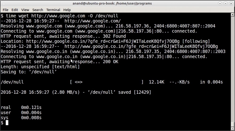
Output of the time command on fetching a web page from the internet via wget
See that it shows three classes of time output, namely real, user, and sys. It is important to know the distinction between these three so let us look at them briefly:
real: Real time is the actual wall-clock time that elapsed for the operation. This is the time of the operation from start to finish. It will include any time the process sleeps or spends blocked—such as time taken for I/O to complete.User: User time is the amount of actual CPU time spent within the process in user mode (outside the kernel). Any sleep time or time spent in waiting such as I/O doesn't add to the user time.Sys: System time is the amount of CPU time spent on executing system calls within the kernel for the program. This counts only those functions that execute in kernel space such as privileged system calls. It doesn't count any system calls that execute in user space (which is counted inUser).
The total CPU time spent by a process is user + sys time. The real or wall-clock time is the time mostly measured by simple time counters.
In Python, it is not very difficult to write a simple function that serves as a context manager for blocks of code whose execution time you want to measure.
But first we need a program whose performance we can measure.
Take a look at the following steps to learn how to use a context manager for measuring time:
- Let us write a program that calculates the common elements between two sequences as a test program. Here is the code:
def common_items(seq1, seq2): """ Find common items between two sequences """ common = [] for item in seq1: if item in seq2: common.append(item) return common - Let us write a simple context-manager timer to time this code. For timing we will use
perf_counterof thetimemodule, which gives the time to the most precise resolution for short durations:from time import perf_counter as timer_func from contextlib import contextmanager @contextmanager def timer(): """ A simple timing function for routines """ try: start = timer_func() yield except Exception as e: print(e) raise finally: end = timer_func() print ('Time spent=>',1000.0*(end – start),'ms.') - Let us time the function for some simple input data. For this a
testfunction is useful that generates random data, given an input size:def test(n): """ Generate test data for numerical lists given input size """ a1=random.sample(range(0, 2*n), n) a2=random.sample(range(0, 2*n), n) return a1, a2Here is the output of the
timermethod on thetestfunction on the Python interactive interpreter:>>> with timer() as t: ... common = common_items(*test(100)) ... Time spent=> 2.0268699999999864 ms.
- In fact both test data generation and testing can be combined in the same function to make it easy to test and generate data for a range of input sizes:
def test(n, func): """ Generate test data and perform test on a given function """ a1=random.sample(range(0, 2*n), n) a2=random.sample(range(0, 2*n), n) with timer() as t: result = func(a1, a2) - Now let us measure the time taken for different ranges of input sizes in the Python interactive console:
>>> test(100, common_items)
    Time spent=> 0.6799279999999963 ms.
>>> test(200, common_items)
    Time spent=> 2.7455590000000085 ms.
>>> test(400, common_items)
    Time spent=> 11.440810000000024 ms.
>>> test(500, common_items)
    Time spent=> 16.83928100000001 ms.
>>> test(800, common_items)
    Time spent=> 21.15130400000004 ms.
>>> test(1000, common_items)
    Time spent=> 13.200749999999983 ms.
Oops, the time spent for
1000items is less than that for800! How's that possible? Let's try again:>>> test(800, common_items) Time spent=> 8.328282999999992 ms. >>> test(1000, common_items) Time spent=> 34.85899500000001 ms.Now the time spent for
800items seems to be lesser than that for400and500. And time spent for1000items has increased to more than twice what it was before.The reason is that our input data is random, which means it will sometimes have a lot of common items—which takes more time—and sometimes have much fewer. Hence on subsequent calls the time taken can show a range of values.
In other words, our timing function is useful to get a rough picture, but not very useful when it comes to getting the true statistical measure of time taken for program execution, which is more important.
- For this we need to run the timer many times and take an average. This is somewhat similar to the amortized analysis of algorithms, which takes into account both the lower end and upper end of the time taken for executing algorithms and gives the programmer a realistic estimate of the average time spent.
Python comes with such a module, which helps to perform such timing analysis, in its standard library, namely the timeit module. Let us look at this module in the next section.
The timeit module in the Python standard library allows the programmer to measure the time taken to execute small code snippets. The code snippets can be a Python statement, an expression, or a function.
The simplest way to use the timeit module is to execute it as a module in the Python command line.
For example, here is timing data for some simple Python inline code measuring the performance of a list comprehension calculating squares of numbers in a range:
$ python3 -m timeit '[x*x for x in range(100)]'
100000 loops, best of 3: 5.5 usec per loop

$ python3 -m timeit '[x*x for x in range(1000)]'
10000 loops, best of 3: 56.5 usec per loop

$ python3 -m timeit '[x*x for x in range(10000)]'
1000 loops, best of 3: 623 usec per loop
The result shows the time taken for execution of the code snippet. When run on the command line, the timeit module automatically determines the number of cycles to run the code and also calculates the average time spent in a single execution.
Here is how to use the timeit module on the Python interpreter in a similar manner:
>>> 1000000.0*timeit.timeit('[x*x for x in range(100)]', number=100000)/100000.0
6.007622049946804

>>> 1000000.0*timeit.timeit('[x*x for x in range(1000)]', number=10000)/10000.0
58.761584300373215The timeit module uses a Timer class behind the scenes. The class can be made use of directly as well as for finer control.
When using this class, timeit becomes a method of the instance of the class to which the number of cycles is passed as an argument.
The Timer class constructor also accepts an optional setup argument, which sets up the code for the Timer class. This can contain statements for importing the module that contains the function, setting up globals, and so on. It accepts multiple statements separated by semi-colons.
Let us rewrite our
test function to test the common items between two sequences. Now that we are going to use the timeit module, we can remove the context manager timer from the code. We will also hardcode the call to common_items in the function.
Note
We also need to create the random input outside the test function otherwise the time taken for it will add to the test function's time and corrupt our results.
Hence we need to move the variables out as globals in the module and write a setup function, which will generate the data for us as a first step.
Our rewritten test function looks like this:
def test():
    """ Testing the common_items function """

    common = common_items(a1, a2)
The setup function with the global variables looks like this:
# Global lists for storing test data
a1, a2 = [], []

def setup(n):
    """ Setup data for test function """

    global a1, a2
    a1=random.sample(range(0, 2*n), n)
    a2=random.sample(range(0, 2*n), n)
Let's assume the module containing both the test and common_items functions is named common_items.py.
The timer test can now be run as follows:
>>> t=timeit.Timer('test()', 'from common_items import test,setup; setup(100)')
>>> 1000000.0*t.timeit(number=10000)/10000
116.58759460115107
So the time taken for a range of 100 numbers is around 117 usec (0.12 microseconds) on average.
Executing it now for a few other ranges of input sizes gives the following output:
>>> t=timeit.Timer('test()','from common_items import test,setup; setup(200)')
>>> 1000000.0*t.timeit(number=10000)/10000
482.8089299000567

>>> t=timeit.Timer('test()','from common_items import test,setup; setup(400)')
>>> 1000000.0*t.timeit(number=10000)/10000
1919.577144399227

>>> t=timeit.Timer('test()','from common_items import test,setup; setup(800)')
>>> 1000000.0*t.timeit(number=1000)/1000
7822.607815993251

>>> t=timeit.Timer('test()','from common_items import test,setup; setup(1000)')
>>> 1000000.0*t.timeit(number=1000)/1000
12394.932234004957
So the maximum time taken for this test run is 12.4 microseconds for an input size of 1000 items.
Is it possible to find out from these results what the time-performance complexity of our function is? Let us try plotting it in a graph and see the results.
The matplotlib library is very useful in plotting graphs in Python for any type of input data. We just need the following simple piece of code for this to work:
import matplotlib.pyplot as plt

def plot(xdata, ydata):
    """ Plot a range of ydata (on y-axis) against xdata (on x-axis) """

    plt.plot(xdata, ydata)
    plt.show()
The preceding code gives you the following output:
This is our x data.
>>> xdata = [100, 200, 400, 800, 1000]
This is the corresponding y data.
>>> ydata = [117,483,1920,7823,12395]
>>> plot(xdata, ydata)
Take a look at the following graph:
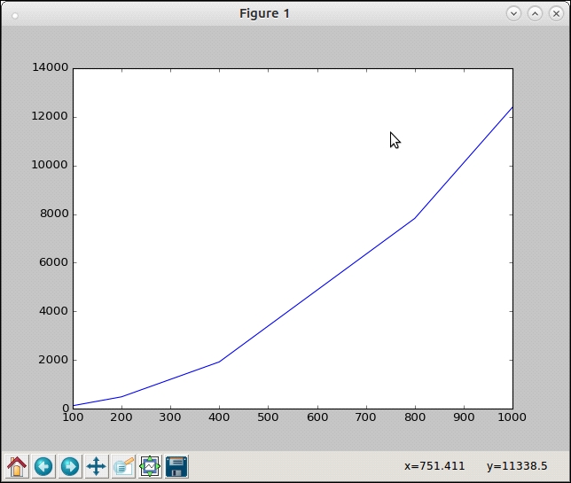
Plot of the input range versus time taken for the common_items function
This is clearly not linear, yet of course not quadratic (in comparison with the figure on Big-O notations). Let us try and plot a graph of O(n*log(n)) superimposed on the current plot to see if there's a match.
Since we now need two series of ydata, we need another slightly modified function:
def plot_many(xdata, ydatas):
    """ Plot a sequence of ydatas (on y-axis) against xdata (on x-axis) """

    for ydata in ydatas:
        plt.plot(xdata, ydata)
    plt.show()
The preceding code gives you the following output:
>>> ydata2=map(lambda x: x*math.log(x, 2), input)

>>> plot_many(xdata, [ydata2, ydata])
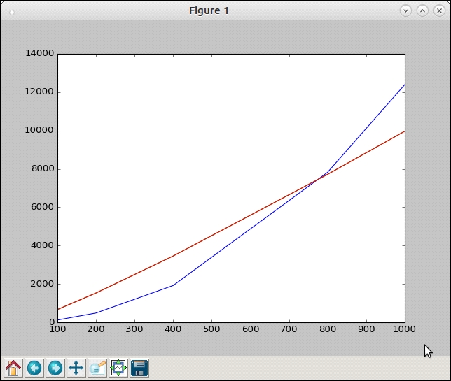
Plot of time complexity of common_items superimposed on the plot of y = x*log(x)
The superimposed plot shows that the function is a close match for the n*log(n) order, if not exactly the same. So our current implementation's complexity seems to be roughly O(n*log(n)).
Now that we've done the performance analysis, let us see if we can rewrite our routine to perform better.
Here is the current code:
def common_items(seq1, seq2):
    """ Find common items between two sequences """

    common = []
    for item in seq1:
        if item in seq2:
            common.append(item)

    return common
The routine first does a pass over an outer for loop (of size n) and does a check in a sequence (also of size n) for the item. Now the second search is also of time complexity n on average.
However, some items would be found immediately and some items would take linear time (k) where 1<k<n. On average, the distribution would be somewhere in between, which is why the code has an average complexity approximating O(n*log(n)).
A quick analysis will tell you that the inner search can be avoided by converting the outer sequence to a dictionary, setting values to 1. The inner search will be replaced with a loop on the second sequence that increments values by 1.
In the end, all common items will have a value greater than 1 in the new dictionary.
The new code is as follows:
def common_items(seq1, seq2):
    """ Find common items between two sequences, version 2.0 """

    seq_dict1 = {item:1 for item in seq1}

    for item in seq2:
        try:
            seq_dict1[item] += 1
        except KeyError:
            pass

    # Common items will have value > 1
    return [item[0] for item in seq_dict1.items() if item[1]>1]
With this change, the timer gives the following updated results:
>>> t=timeit.Timer('test()','from common_items import test,setup; setup(100)')
>>> 1000000.0*t.timeit(number=10000)/10000
35.777671200048644

>>> t=timeit.Timer('test()','from common_items import test,setup; setup(200)')
>>> 1000000.0*t.timeit(number=10000)/10000
65.20369809877593

>>> t=timeit.Timer('test()','from common_items import test,setup; setup(400)')
>>> 1000000.0*t.timeit(number=10000)/10000
139.67061050061602

>>> t=timeit.Timer('test()','from common_items import test,setup; setup(800)')
>>> 1000000.0*t.timeit(number=10000)/10000
287.0645995993982

>>> t=timeit.Timer('test()','from common_items import test,setup; setup(1000)')
>>> 1000000.0*t.timeit(number=10000)/10000
357.764518300246
Let us plot this and superimpose it on an O(n) graph:
>>> input=[100,200,400,800,1000]
>>> ydata=[36,65,140,287,358]

# Note that ydata2 is same as input as we are superimposing with y = x
# graph
>>> ydata2=input
>>> plot.plot_many(xdata, [ydata, ydata2])
Let's take a look at the following graph:
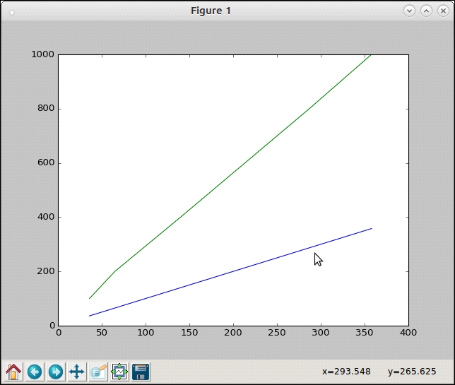
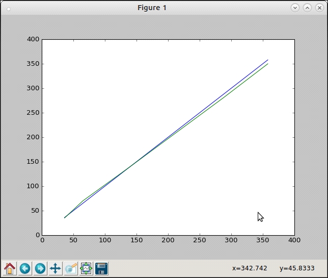
Plot of time taken by common_items function (v2) against y = x graph
The upper green line is the reference y = x graph and the lower blue line is the plot of the time taken by our new function. It is pretty obvious that the time complexity is now linear or O(n).
However, there seems to be a constant factor here as the slopes of the two lines are different. From a quick calculation one can compute this factor as roughly 0.35.
After applying this change, you will get the following output:
>>> input=[100,200,400,800,1000]
>>> ydata=[36,65,140,287,358]

# Adjust ydata2 with the constant factor
>>> ydata2=map(lambda x: 0.35*x, input)
>>> plot.plot_many(xdata, [ydata, ydata2])
The output can be seen in the following graph as follows:
Plot of time taken by common_items function (v2) against y = 0.35*x graph
You can see that the plots pretty much superimpose on each other. So our function is now performing at O(c*n) where c ~= 0.35.
The Timer module by default uses the perf_counter function of the time module as the default timer function. As mentioned earlier, this function returns the wall-clock time spent to the maximum precision for small time durations, hence it will include any sleep time, time spent for I/O, and so on.
This can be made clear by adding a little sleep time to our test function as follows:
def test():
    """ Testing the common_items function using a given input size """

    sleep(0.01)
    common = common_items(a1, a2)
The preceding code will give you the following output:
>>> t=timeit.Timer('test()','from common_items import test,setup; setup(100)')
>>> 1000000.0*t.timeit(number=100)/100
10545.260819926625
The time jumped by as much as 300 times since we are sleeping 0.01 seconds (10 milliseconds) upon every invocation, so the actual time spent on the code is now determined almost completely by the sleep time as the result shows 10545.260819926625 microseconds (or about 10 milliseconds).
Sometimes you may have such sleep times and other blocking or wait times but you want to measure only the actual CPU time taken by the function. To use this, the Timer object can be created using the process_time function of the time module as the timer function.
This can be done by passing in a timer argument when you create the Timer object:
>>> from time import process_time
>>> t=timeit.Timer('test()','from common_items import test,setup;setup(100)', timer=process_time)
>>> 1000000.0*t.timeit(number=100)/100
345.22438
If you now increase the sleep time by a factor of, say, 10, the testing time increases by that factor, but the return value of the timer remains the same.
For example, here is the result when sleeping for 1 second. The output comes after about 100 seconds (since we are iterating 100 times), but notice that the return value (time spent per invocation) doesn't change:
>>> t=timeit.Timer('test()','from common_items import test,setup;setup(100)', timer=process_time)
>>> 1000000.0*t.timeit(number=100)/100
369.8039100000002
Let us move on to profiling next.