
The concurrent.futures module provides high-level concurrent processing using either threads or processes, while asynchronously returning data using future objects.
It provides an executor interface which exposes mainly two methods, which are as follows:
submit: Submits a callable to be executed asynchronously, returning afutureobject representing the execution of the callable.map: Maps a callable to a set of iterables, scheduling the execution asynchronously in thefutureobject. However, this method returns the results of processing directly instead of returning a list of futures.
There are two concrete implementations of the executor interface: ThreadPoolExecutor executes the callable in a pool of threads, and ProcessPoolExecutor does so in a pool of processes.
Here is a simple example of a future object that calculates the factorial of a set of integers asynchronously:
from concurrent.futures import ThreadPoolExecutor, as_completed
import functools
import operator

def factorial(n):
    return functools.reduce(operator.mul, [i for i in range(1, n+1)])

with ThreadPoolExecutor(max_workers=2) as executor:
    future_map = {executor.submit(factorial, n): n for n in range(10, 21)}
    for future in as_completed(future_map):
        num = future_map[future]
        print('Factorial of',num,'is',future.result())
The following is a detailed explanation of the preceding code:
- The
factorialfunction computes the factorial of a given number iteratively by usingfunctools.reduceand the multiplication operator - We create an executor with two workers, and submit the numbers (from 10 to 20) to it via its
submitmethod - The submission is done via a dictionary comprehension, returning a dictionary with the future as the key and the number as the value
- We iterate through the completed futures, which have been computed, using the
as_completedmethod of theconcurrent.futuresmodule - The result is printed by fetching the future's result via the
resultmethod
When executed, the program prints its output, rather in order, as shown in the next screenshot:
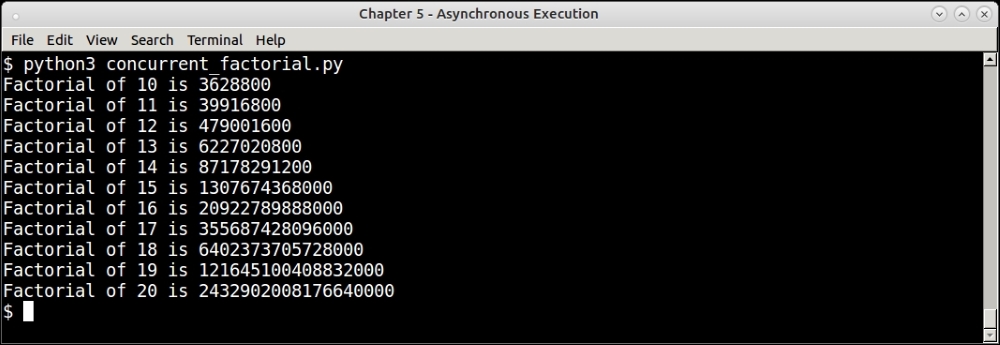
Output of concurrent futures factorial program
In our earlier discussion of threads, we used the example of the generation of thumbnails for random images from the Web to demonstrate how to work with threads, and process information.
In this example, we will do something similar. Here, rather than processing random image URLs from the Web, we will load images from disk, and convert them to thumbnails using the concurrent.futures function.
We will reuse our thumbnail creation function from before. On top of that, we will add concurrent processing.
First, here are the imports:
import os
import sys
import mimetypes
from concurrent.futures import ThreadPoolExecutor, ProcessPoolExecutor, as_completed
Here is our familiar thumbnail creation function:
def thumbnail_image(filename, size=(64,64), format='.png'):
    """ Convert image thumbnails, given a filename """

    try:
        im=Image.open(filename)
        im.thumbnail(size, Image.ANTIALIAS)

        basename = os.path.basename(filename)
        thumb_filename = os.path.join('thumbs',
            basename.rsplit('.')[0] + '_thumb.png')
        im.save(thumb_filename)
        print('Saved',thumb_filename)
        return True

    except Exception as e:
        print('Error converting file',filename)
        return False
We will process images from a specific folder—in this case, the Pictures subdirectory of the home folder. To process this, we will need an iterator that yields image filenames. We have written one next with the help of the os.walk function:
def directory_walker(start_dir):
    """ Walk a directory and generate list of valid images """

    for root,dirs,files in os.walk(os.path.expanduser(start_dir)):
        for f in files:
            filename = os.path.join(root,f)
            # Only process if it's a type of image
            file_type = mimetypes.guess_type(filename.lower())[0]
            if file_type != None and file_type.startswith('image/'):
                yield filename
As you can see, the preceding function is a generator.
Here is the main calling code, which sets up an executor and runs it over the folder:
    root_dir = os.path.expanduser('~/Pictures/')
    if '--process' in sys.argv:
        executor = ProcessPoolExecutor(max_workers=10)
    else:
        executor = ThreadPoolExecutor(max_workers=10)

    with executor:
        future_map = {executor.submit(thumbnail_image, filename): filename for filename in directory_walker(root_dir)}
        for future in as_completed(future_map):
            num = future_map[future]
            status = future.result()
            if status:
                print('Thumbnail of',future_map[future],'saved')
The preceding code uses the same technique of submitting arguments to a function asynchronously, saving the resultant futures in a dictionary and then processing the result as and when the futures are finished, in a loop.
To change the executor to use processes, one simply needs to replace ThreadPoolExecutor with ProcessPoolExecutor; the rest of the code remains the same. We have provided a simple command-line flag, --process, to make this easy.
Here is an output of a sample run of the program using both thread and process pools on the ~/Pictures folder—generating around 2000+ images in roughly the same time.
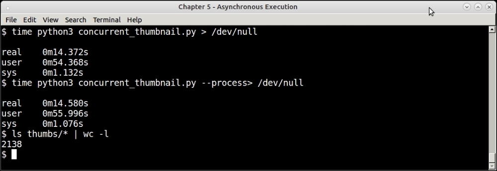
Output of concurrent futures disk thumbnail program—using thread and process executor
We are at the end of our discussion of concurrency techniques in Python. We discussed threads, processes, asynchronous I/O, and concurrent futures. Naturally, a question arises—when to pick what?
This question has been already answered for the choice between threads and processes, where the decision is mostly influenced by the GIL.
Here are some rough guidelines for picking your concurrency options.
- Concurrent futures versus multiprocessing: Concurrent futures provide an elegant way to parallelize your tasks using either a thread or process pool executor. Hence, it is ideal if the underlying application has similar scalability metrics with either threads or processes, since it's very easy to switch from one to the other as we've seen in a previous example. Concurrent futures can be chosen also when the result of the operation needn't be immediately available. Concurrent futures is a good option when the data can be finely parallelized and the operation can be executed asynchronously, and when the operations involve simple callables without requiring complex synchronization techniques.
Multiprocessing should be chosen if the concurrent execution is more complex, and not just based on data parallelism, but has aspects like synchronization, shared memory, and so on. For example, if the program requires processes, synchronization primitives, and IPC, the only way to truly scale up then, is to write a concurrent program using the primitives provided by the multiprocessing module.
Similarly when your multithreaded logic involves simple parallelization of data across multiple tasks, one can choose concurrent futures with a thread pool. However if there is a lot of shared state to be managed with complex thread synchronization objects—one has to use thread objects and switch to multiple threads using
threadingmodule to get finer control of the state. - Asynchronous I/O vs threaded concurrency: When your program doesn't need true concurrency (parallelism), but is dependent more on asynchronous processing and callbacks, then
asynciois the way to go. Asyncio is a good choice when there are lot of waits or sleep cycles involved in the application, such as waiting for user input, waiting for I/O, and so on, and one needs to take advantage of such wait or sleep times by yielding to other tasks via co-routines. Asyncio is not suitable for CPU-heavy concurrent processing, or for tasks involving true data parallelism.AsyncIO seems to be suitable for request-response loops, where a lot of I/O happens – so its good for writing web application servers which do not have real-time data requirements.
You can use the points just listed as rough guidelines when deciding on the correct concurrency package for your applications.
Apart from the standard library modules that we've discussed so far, Python is also rich in its ecosystem of third-party libraries, which support parallel processing in symmetric multi-processing (SMP) or multi-core systems.
We will take a look at a couple of such packages, that are somewhat distinct and present some interesting features.
joblib is a package that provides a wrapper over multiprocessing to execute code in loops in parallel. The code is written as a generator expression, and interpreted to execute in parallel over CPU cores using multiprocessing modules behind the scenes.
For example, take the following code which calculates square roots for first 10 numbers:
>>> [i ** 0.5 for i in range(1, 11)]
[1.0, 1.4142135623730951, 1.7320508075688772, 2.0, 2.23606797749979, 2.449489742783178, 2.6457513110645907, 2.8284271247461903, 3.0, 3.1622776601683795]
This preceding code can be converted to run on two CPU cores by the following:
>>> import math
>>> from joblib import Parallel, delayed
    [1.0, 1.4142135623730951, 1.7320508075688772, 2.0, 2.23606797749979, 2.449489742783178, 2.6457513110645907, 2.8284271247461903, 3.0, 3.1622776601683795]
Here is another example: this is our primality checker that we had written earlier to run using multiprocessing, rewritten to use the joblib package:
# prime_joblib.py
from joblib import Parallel, delayed

def is_prime(n):
    """ Check for input number primality """

    for i in range(3, int(n**0.5+1), 2):
        if n % i == 0:
            print(n,'is not prime')
            return False

    print(n,'is prime')
    return True

if __name__ == "__main__":
    numbers = [1297337, 1116281, 104395303, 472882027, 533000389, 817504243, 982451653, 112272535095293, 115280095190773, 1099726899285419]*100
    Parallel(n_jobs=10)(delayed(is_prime)(i) for i in numbers)
If you execute and time the preceding code, you will find the performance metrics very similar to that of the version using multiprocessing.
OpenMP is an open API, which supports shared memory multiprocessing in C/C++ and Fortran. It uses special work-sharing constructs such as pragmas (special instructions to compilers) indicating how to split work among threads or processes.
For example, the following C code using the OpenMP API indicates that the array should be initialized in parallel using multiple threads:
int parallel(int argc, char **argv)
{
    int array[100000];

    #pragma omp parallel for
    for (int i = 0; i < 100000; i++) {
array[i] = i * i;
	}

return 0;
}
PyMP is inspired by the idea behind OpenMP, but uses the fork system call to parallelize code executing in expressions such as for loops across processes. For this, PyMP also provides support for shared data structures such as lists and dictionaries, and also provides a wrapper for numpy arrays.
We will look at an interesting and exotic example—that of fractals—to illustrate how PyMP can be used to parallelize code and obtain performance improvement.
The following is the code listing of a very popular class of complex numbers, which when plotted, produces very interesting fractal geometries, namely, the Mandelbrot set:
# mandelbrot.py
import sys
import argparse
from PIL import Image

def mandelbrot_calc_row(y, w, h, image, max_iteration = 1000):
    """ Calculate one row of the Mandelbrot set with size wxh """

    y0 = y * (2/float(h)) - 1 # rescale to -1 to 1

    for x in range(w):
        x0 = x * (3.5/float(w)) - 2.5 # rescale to -2.5 to 1

        i, z = 0, 0 + 0j
        c = complex(x0, y0)
        while abs(z) < 2 and i < max_iteration:
            z = z**2 + c
            i += 1

        # Color scheme is that of Julia sets
        color = (i % 8 * 32, i % 16 * 16, i % 32 * 8)
        image.putpixel((x, y), color)


def mandelbrot_calc_set(w, h, max_iteration=10000, output='mandelbrot.png'):
    """ Calculate a mandelbrot set given the width, height and
    maximum number of iterations """

    image = Image.new("RGB", (w, h))

    for y in range(h):
        mandelbrot_calc_row(y, w, h, image, max_iteration)

    image.save(output, "PNG")

if __name__ == "__main__":
    parser = argparse.ArgumentParser(prog='mandelbrot', description='Mandelbrot fractal generator')
    parser.add_argument('-W','--width',help='Width of the image',type=int, default=640)
    parser.add_argument('-H','--height',help='Height of the image',type=int, default=480)
    parser.add_argument('-n','--niter',help='Number of iterations',type=int, default=1000)
    parser.add_argument('-o','--output',help='Name of output image file',default='mandelbrot.png')

    args = parser.parse_args()
    print('Creating Mandelbrot set with size %(width)sx%(height)s, #iterations=%(niter)s' % args.__dict__)
    mandelbrot_calc_set(args.width, args.height, max_iteration=args.niter, output=args.output)
The preceding code calculates a Mandelbrot set using a certain number of c and a variable geometry (width x height). It is complete with argument parsing to produce fractal images of varying geometries, and supports different iterations.
How does it work ? Here is an explanation of the code .
- The
mandelbrot_calc_rowfunction calculates a row of the Mandelbrot set for a certain value of the y coordinate for a certain number of maximum iterations. The pixel color values for the entire row, from0to widthwfor the x coordinate, is calculated. The pixel values are put into theImageobject that is passed to this function. - The
mandelbrot_calc_setfunction calls themandelbrot_calc_rowfunction for all values of the y coordinate ranging from0to the heighthof the image. AnImageobject (via the Pillow library) is created for the given geometry (width x height), and filled with pixel values. Finally, we save this image to a file, and we've got our fractal!
Without further ado, let's see the code in action.
Here is the image that our Mandelbrot program produces for the default number of iterations namely 1000.

Mandelbrot set fractal image for 1,000 iterations
Here is the time it takes to create this image.
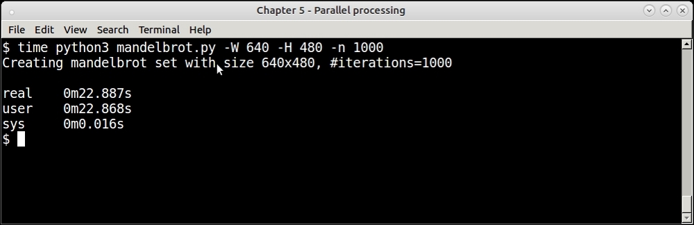
Timing of single process Mandelbrot program—for 1,000 iterations
However, if you increase the number of iterations—the single process version slows down quite a bit. Here is the output when we increase the number of iterations by 10X—for 10,000 iterations:
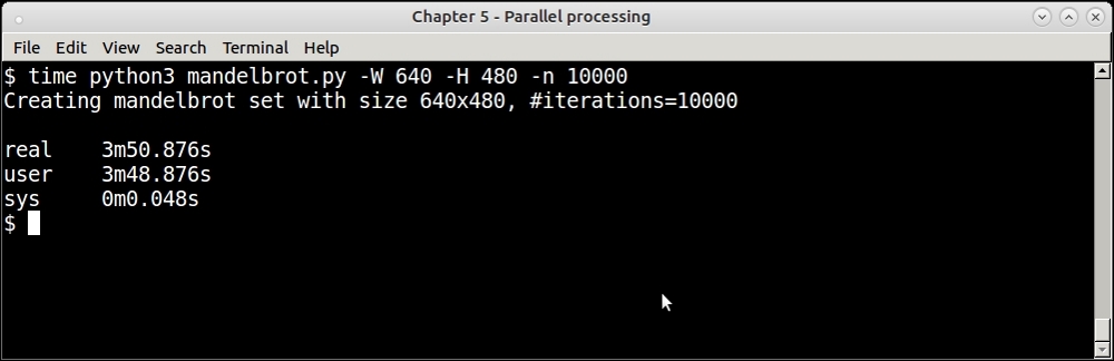
Timing of single process Mandelbrot program—for 10,000 iterations
If we look at the code, we can see that there is an outer for loop in the mandelbrot_calc_set function, which sets things in motion. It calls mandelbrot_calc_row for each row of the image ranging from 0 to the height of the function, varied by the y coordinate.
Since each invocation of the mandelbrot_calc_row function calculates one row of the image, it naturally fits into a data parallel problem, and can be parallelized sufficiently easily.
In the next section, we will see how to do this using PyMP.
We will use PyMP to parallelize the outer for loop across many processes in a rewrite of the previous simple implementation of the Mandelbrot set, to take advantage of the inherent data parallelism in the solution.
Here is the PyMP version of the two functions of the Mandelbrot program. The rest of the code remains the same.
# mandelbrot_mp.py
import sys
from PIL import Image
import pymp
import argparse


def mandelbrot_calc_row(y, w, h, image_rows, max_iteration = 1000):
    """ Calculate one row of the mandelbrot set with size wxh """

    y0 = y * (2/float(h)) - 1 # rescale to -1 to 1

    for x in range(w):
        x0 = x * (3.5/float(w)) - 2.5 # rescale to -2.5 to 1

        i, z = 0, 0 + 0j
        c = complex(x0, y0)
        while abs(z) < 2 and i < max_iteration:
            z = z**2 + c
            i += 1

        color = (i % 8 * 32, i % 16 * 16, i % 32 * 8)
        image_rows[y*w + x] = color


def mandelbrot_calc_set(w, h, max_iteration=10000, output='mandelbrot_mp.png'):
    """ Calculate a mandelbrot set given the width, height and
    maximum number of iterations """

    image = Image.new("RGB", (w, h))
    image_rows = pymp.shared.dict()

    with pymp.Parallel(4) as p:
        for y in p.range(0, h):
            mandelbrot_calc_row(y, w, h, image_rows, max_iteration)

    for i in range(w*h):
        x,y = i % w, i // w
        image.putpixel((x,y), image_rows[i])

    image.save(output, "PNG")
    print('Saved to',output)
The rewrite mainly involved converting the code to one that builds the Mandelbrot image line by line, each line of data being computed separately and in a way that it can be computed in parallel—in a separate process.
- In the single process version, we put the pixel values directly in the image in the
mandelbrot_calc_rowfunction. However, since the new code executes this function in parallel processes, we cannot modify the image data in it directly. Instead, the new code passes a shared dictionary to the function, and it sets the pixel color values in it using the location askeyand the pixel RGB value asvalue. - A new shared data structure—a shared dictionary—is hence added to the
mandelbrot_calc_setfunction, which is finally iterated over, and the pixel data, filled, in theImageobject, which is then saved to the final output. - We use four
PyMPparallel processes, as the machine has four CPU cores, using a with context and enclosing the outer for loop inside it. This causes the code to execute in parallel in four cores, each core calculating approximately 25% of the rows. The final data is written to the image in the main process.
Here is the result timing of the PyMP version of the code:
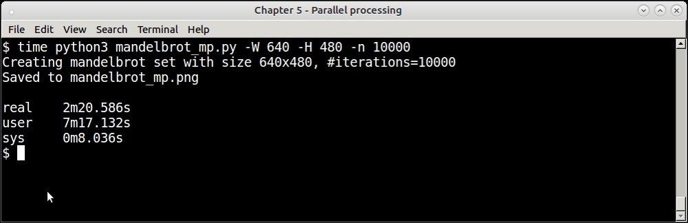
Timing of parallel process Mandelbrot program using PyMP—for 10000 iterations
The program is about 33% faster in real time. In terms of CPU usage, you can see that the PyMP version has a higher ratio of user CPU time to real CPU time, indicating a higher usage of the CPU by the processes than the single process version.
Note
We can write an even more efficient version of the program by avoiding the shared data structure image_rows which is used to keep the pixel values of the image. This version however uses that to show the features of PyMP. The code archives of this book contain two more versions of the program—one that uses multiprocessing and another that uses PyMP without the shared dictionary.
This is the output fractal image produced by this run of the program:

Mandelbrot set fractal image for 10000 iterations using PyMP
You can observe that the colors are different, and this image provides more detail and a finer structure than the previous one due to the increased number of iterations.