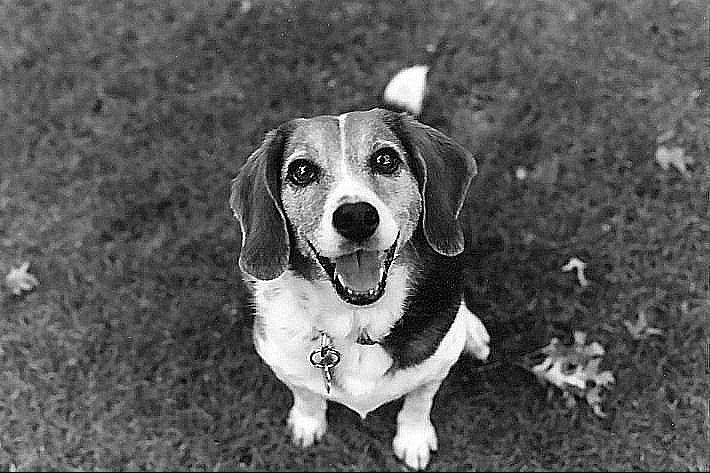
When we feed an image as input, it will actually be converted to a matrix of pixel values. These pixel values range from 0 to 255 and the dimensions of this matrix will be [image height * image width * number of channels]. If the input image is 64 x 64 in size, then the pixel matrix dimension would be 64 x 64 x 3, where the 3 refers to the channel number. A grayscale image has 1 channel and color images have 3 channels (RGB). Look at the following photograph. When this image is fed as an input, it will be converted into a matrix of pixel values, which we will see in a moment. For better understanding, we will consider the grayscale image since grayscale images have 1 channel and so we will get the 2D matrix.

The input image is as follows:

Now, let's see the matrix value in the following graphic:

So, this is how the image is represented by a matrix. What happens next? How does the network identify the image from this pixel's values? Now, we introduce an operation called convolution. It is used to extract important features from the image so that we can understand what the image is all about. Let's say we have the image of a dog; what do you think the features of this image are, which will help us to understand that this is an image of a dog? We can say body structure, face, legs, tail, and so on. Convolution operations will help the network to learn those features which characterize the dog. Now, we will see how exactly the convolution operation is performed to extract features from the image. 

As we know, every image is represented by a matrix. Let's suppose we have a pixel matrix of the dog image, and let's call this matrix an input matrix. We will also consider another n x n matrix called filter, as shown in the following diagram:

Now, this filter will slide over our input matrix by one pixel and will perform element-wise multiplication, producing a single number. Confused? Look at the following diagram:

That is, (13*0) + (8*1) + (18*0) + (5*1) + (3*1) + (1*1) + (1*0) + (9*0) + (0*1) = 17.

Similarly, we move our filter matrix over the input matrix by one pixel and perform element-wise multiplication:

That is, (8*0) + (18*1) + (63*0) + (3*1) + (1*1) + (2*1) + (9*0) + (0*0) + (7*1) = 31.

The filter matrix will slide over the entire input matrix, perform element-wise multiplication, and produce a new matrix called a feature map or activation map. This operation is known as convolution as shown in the following diagram:

 The following output shows an actual and convolved image: 

You can see that our filter has detected an edge in the actual image and produced a convolved image. Similarly, different filters are used to extract different features from the image.

For example, if we use a filter matrix, say a sharpen filter , then our convolved image will look as follows:

Thus, filters are responsible for extracting features from the actual image by performing a convolutional operation. There will be more than one filter for extracting different features of the image that produces the feature maps. The depth of the feature map is the number of the filters we use. If we use 5 filters to extract features and produce 5 feature maps, then the depth of the feature map is 5 shown as follows:

When we have many filters, our network will better understand the image by extracting many features. While building our CNN, we don't have to specify the values for this filter matrix. The optimal values for this filter will be learned during the training process. However, we have to specify the number of filters and dimensions of the filters we want to use.

We can slide over the input matrix by one pixel with the filter and performed convolution operation. Not only can we slide by one pixel; we can also slide over an input matrix by any number of pixels. The number of pixels we slide over the input matrix by in the filter matrix is called strides. 

But what happens when the sliding window (filter matrix) reaches the border of the image? In that case, we pad the input matrix with zero so that we can apply a filter on the image's edges. Padding with zeros on the image is called same padding, or wide convolutional or zero padding illustrated as follows:

Instead of padding them with zeros, we can also simply discard that region. This is known as valid padding or narrow convolution illustrated as follows:

After performing the convolution operation, we apply the ReLU activation function to introduce nonlinearity.