In value iteration, we start off with a random value function. Obviously, the random value function might not be an optimal one, so we look for a new improved value function in iterative fashion until we find the optimal value function. Once we find the optimal value function, we can easily derive an optimal policy from it:

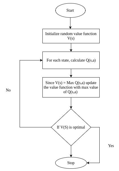
The steps involved in the value iteration are as follows:

1. First, we initialize the random value function, that is, the random value for each state.
2. Then we compute the Q function for all state action pairs of Q(s, a).
3. Then we update our value function with the max value from Q(s,a).
4. We repeat these steps until the change in the value function is very small.

Let us understand it intuitively by performing value iteration manually, step by step.

Consider the grid shown here. Let us say we are in state A and our goal is to reach state C without visiting state B, and we have two actions, 0—left/right and 1—up/down: 

Can you think of what will be the optimal policy here? The optimal policy here will be the one that tells us to perform action 1 in the state A so that we can reach C without visiting B. How can we find this optimal policy? Let us see that now:

 Initialize the random value function, that is, a random values for all the states. Let us assign 0 to all the states:

Let's calculate the Q value for all state action pairs.

The Q value tells us the value of an action in each state. First, let us compute the Q value for state A. Recall the equation of the Q function. For calculating, we need transition and reward probabilities. Let us consider the transition and reward probability for state A as follows:

The Q function for the state A can be calculated as follows:

Q(s,a) =  Transition probability * ( Reward probability + gamma * value_of_next_state)

Here, gamma is the discount factor; we will consider it as 1.

Q value for state A and action 0:

Q(A,0) = (0.1 * (0+0) ) +  (0.4 * (-1.0+0) ) + (0.3 * (1.0+0) )

Q(A,0) = -0.1

Now we will compute the Q value for state A and action 1:

Q(A,1) = (0.3 * (0+0)) + (0.1 * (-2.0 + 0)) + (0.5 * (1.0 + 0))

Q(A,1) = 0.3

Now we will update this in the Q table as follows:

Update the value function as the max value from Q(s,a).

If you look at the preceding Q function, Q(A,1) has a higher value than Q(A,0) so we will update the value of state A as Q(A,1):

Similarly, we compute the Q value for all state-action pairs and update the value function of each state by taking the Q value that has the highest state action value. Our updated value function looks like the following. This is the result of the first iteration:

We repeat this steps for several iterations. That is, we repeat step 2 to step 3 (in each iteration while calculating the Q value, we use the updated value function instead of the same randomly initialized value function).

This is the result of the second iteration:

This is the result of the third iteration:

But when do we stop this? We will stop when the change in the value between each iteration is small; if you look at iteration two and three, there is not much of a change in the value function. Given this condition, we stop iterating and consider it an optimal value function.

Okay, now that we have found the optimal value function, how can we derive the optimal policy? 

It is very simple. We compute the Q function with our final optimal value function. Let us say our computed Q function looks like the following:

From this Q function, we pick up actions in each state that have maximal value. At state A, we have a maximum value for action 1, which is our optimal policy. So if we perform action 1 in state A we can reach C without visiting B.