
For this chapter, a CNN was trained on the dataset that was used and made available from the research paper How Do Humans Sketch Objects? by Mathias Eitz, James Hays, and Marc Alexa. The paper, presented at SIGGRAPH in 2012, compares the performance of humans classifying sketches to that of a machine. The dataset consists of 20,000 sketches evenly distributed across 250 object categories, ranging from airplanes to zebras; a few examples are shown here:

From a perceptual study, they found that humans correctly identified the object category (such as snowman, grapes, and many more) of a sketch 73% of the time. The competitor, their ML model, got it right 56% of the time. Not bad! You can find out more about the research and download the accompanying dataset here at the official web page: http://cybertron.cg.tu-berlin.de/eitz/projects/classifysketch/.
In this project, we will be using a slightly smaller set, with 205 out of the 250 categories; the exact categories can be found in the CSV file /Chapter7/Training/sketch_classes.csv, along with the Jupyter Notebooks used to prepare the data and train the model. The original sketches are available in SVG and PNG formats. Because we're using a CNN, rasterized images (PNG) were used but rescaled from 1111 x 1111 to 256 x 256; this is the expected input of our model. The data was then split into a training and a validation set, using 80% (64 samples from each category) for training and 20% (17 samples from each category) for validation.
The architecture of the network was not too dissimilar to what has been used in previous chapters, with the exception of a larger kernel window used in the first layer to extract the spare features of the sketch, as presented here:
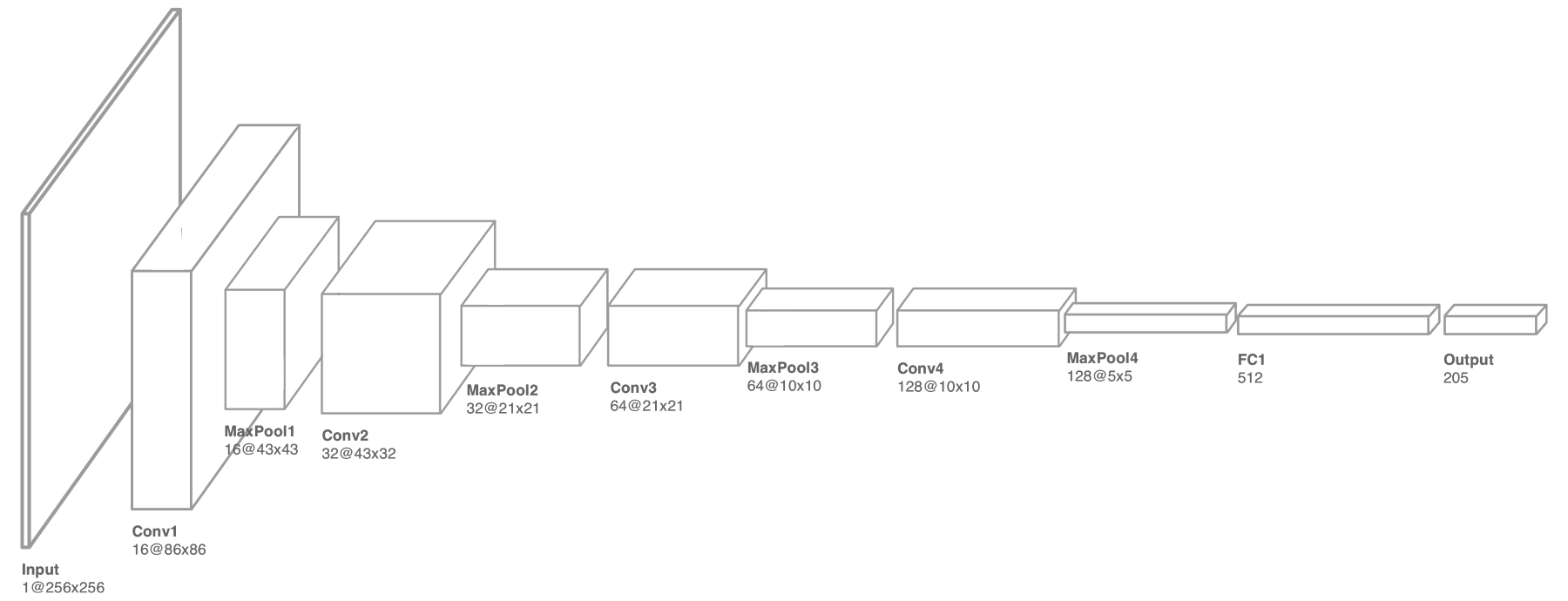
Recall that stacking convolution layers on top of each other allows the model to build up a shared set of high-level patterns that can then be used to perform classification, as opposed to using the raw pixels. The last convolution layer is flattened and then fed into a fully connected layer, where the prediction is finally made. You can think of these fully connected nodes as switches that turn on when certain (high-level) patterns are present in the input, as illustrated in the following diagram. We will return to this concept later on in this chapter when we implement sorting:

After 68 iterations (epochs), the model was able to achieve an accuracy of approximately 65% on the validation data. Not exceptional, but if we consider the top two or three predictions, then this accuracy increases to nearly 90%. The following diagram shows the plots comparing training and validation accuracy, and loss during training:

With our model trained, our next step is to export it using the Core ML Tools made available by Apple (as discussed in previous chapters) and imported into our project.