The development of a volatility model for an asset-return series consists of four steps:

1. Build an ARMA time series model for the financial time series based on the serial dependence revealed by the ACF and PACF.
2. Test the residuals of the model for ARCH/GARCH effects, again relying on the ACF and PACF for the series of the squared residual.
3. Specify a volatility model if serial correlation effects are significant, and jointly estimate the mean and volatility equations.
4. Check the fitted model carefully and refine it if necessary.

The arch library provides several options to estimate volatility-forecasting models. It offers several options to model the expected mean, including a constant mean, the AR(p) model discussed in the section on univariate time series models above as well as more recent heterogeneous autoregressive processes (HAR) that use daily (1 day), weekly (5 days), and monthly (22 days) lags to capture the trading frequencies of short-, medium-, and long-term investors.

The mean models can be jointly defined and estimated with several conditional heteroskedasticity models that include, in addition to ARCH and GARCH, the exponential GARCH (EGARCH) model, which allows for asymmetric effects between positive and negative returns and the heterogeneous ARCH (HARCH) model, which complements the HAR mean model.

We will use daily NASDAQ returns from 1998-2017 to demonstrate the usage of a GARCH model (see the notebook arch_garch_models for details):

nasdaq = web.DataReader('NASDAQCOM', 'fred', '1998', '2017-12-31').squeeze()
nasdaq_returns = np.log(nasdaq).diff().dropna().mul(100) # rescale to facilitate optimization

The rescaled daily return series exhibits only limited autocorrelation, but the squared deviations from the mean do have substantial memory reflected in the slowly-decaying ACF and the PACF high for the first two and cutting off only after the first six lags:

plot_correlogram(nasdaq_returns.sub(nasdaq_returns.mean()).pow(2), lags=120, title='NASDAQ Daily Volatility')

The function plot_correlogram produces the following output:

Hence, we can estimate a GARCH model to capture the linear relationship of past volatilities. We will use rolling 10-year windows to estimate a GARCH(p, q) model with p and q ranging from 1-4 to generate 1-step out-of-sample forecasts. We then compare the RMSE of the predicted volatility relative to the actual squared deviation of the return from its mean to identify the most predictive model. We are using winsorized data to limit the impact of extreme return values reflected in the very high positive skew of the volatility:

trainsize = 10 * 252  # 10 years
data = nasdaq_returns.clip(lower=nasdaq_returns.quantile(.05),
                           upper=nasdaq_returns.quantile(.95))
T = len(nasdaq_returns)
test_results = {}
for p in range(1, 5):
    for q in range(1, 5):
        print(f'{p} | {q}')
        result = []
        for s, t in enumerate(range(trainsize, T-1)):
            train_set = data.iloc[s: t]
            test_set = data.iloc[t+1]  # 1-step ahead forecast
            model = arch_model(y=train_set, p=p, q=q).fit(disp='off')
            forecast = model.forecast(horizon=1)
            mu = forecast.mean.iloc[-1, 0]
            var = forecast.variance.iloc[-1, 0]
            result.append([(test_set-mu)**2, var])
        df = pd.DataFrame(result, columns=['y_true', 'y_pred'])
        test_results[(p, q)] = np.sqrt(mean_squared_error(df.y_true, df.y_pred))

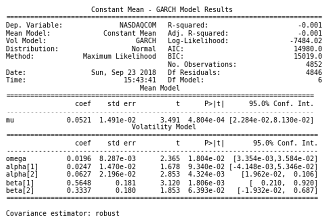
The GARCH(2, 2) model achieves the lowest RMSE (same value as GARCH(4, 2) but with fewer parameters), so we go ahead and estimate this model to inspect the summary:

am = ConstantMean(nasdaq_returns.clip(lower=nasdaq_returns.quantile(.05),
                                      upper=nasdaq_returns.quantile(.95)))
am.volatility = GARCH(2, 0, 2)
am.distribution = Normal()
model = am.fit(update_freq=5)
print(model.summary())

The output shows the maximized log-likelihood as well as the AIC and BIC criteria that are commonly minimized when selecting models based on in-sample performance (see Chapter 7, Linear Models). It also displays the result for the mean model, which in this case is just a constant estimate, as well as the GARCH parameters for the constant omega, the AR parameters, α, and the MA parameters, β, all of which are statistically significant:

Let's now explore models for multiple time series and the concept of cointegration, which will enable a new trading strategy.