Next, we'll look at the alternative computation using Singular Value Decomposition (SVD). This algorithm is slower when the number of observations is greater than the number of features (the typical case), but yields better numerical stability, especially when some of the features are strongly correlated (often the reason to use PCA in the first place).

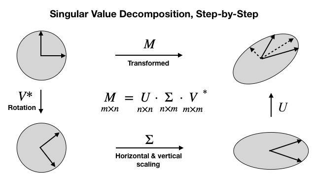
SVD generalizes the eigendecomposition that we just applied to the square and symmetric covariance matrix to the more general case of m x n rectangular matrices. It has the form shown at the center of the following diagram. The diagonal values of Σ are the singular values, and the transpose of V* contains the principal components as column vectors:

In this case, we need to make sure our data is centered with mean zero (the computation of the covariance preceding took care of this):

n_features = data.shape[1]
data_ = data - data.mean(axis=0
Using the centered data, we compute the singular value decomposition:
U, s, Vt = svd(data_)
U.shape, s.shape, Vt.shape
((100, 100), (3,), (3, 3))
We can convert the vector s that only contains the singular values into an nxm matrix and show that the decomposition works:
S = np.zeros_like(data_)
S[:n_features, :n_features] = np.diag(s)
S.shape
(100, 3)

We find that the decomposition does indeed reproduce the standardized data:

np.allclose(data_, U.dot(S).dot(Vt))
True

Lastly, we confirm that the columns of the transpose of V* contain the principal components:

np.allclose(np.abs(C), np.abs(Vt.T))
True

In the next section, we show how sklearn implements PCA.