We are going through the process of implementing an example of a pair trading strategy. The first step is to determine the pairs that have a high correlation. This can be based on the underlying economic relationship (for example, companies having similar business plans) or also a financial product created out of some others, such as ETF. Once we figure out which symbols are correlated, we will create the trading signals based on the value of these correlations. The correlation value can be the Pearson's coefficient, or a Z-score.

In case of a temporary divergence, the outperforming stock (the stock that moved up) would have been sold and the underperforming stock (the stock that moved down) would have been purchased. If the two stocks converge by either the outperforming stock moving back down or the underperforming stock moving back up, or both, you will make money in such cases. You won't make money in the event that both stocks move up or down together with no change in the spread between them. Pairs trading is a market neutral trading strategy as it allows traders to profit from changing market conditions:

1. Let's begin by creating a function establishing cointegration between pairs, as shown in the following code. This function takes as inputs a list of financial instruments and calculates the cointegration values of these symbols. The values are stored in a matrix. We will use this matrix to display a heatmap:

def find_cointegrated_pairs(data):
     n = data.shape[1]
     pvalue_matrix = np.ones((n, n))
     keys = data.keys()
     pairs = []
     for i in range(n):
         for j in range(i+1, n):
             result = coint(data[keys[i]], data[keys[j]])
             pvalue_matrix[i, j] = result[1]
             if result[1] < 0.02:
                 pairs.append((keys[i], keys[j]))
     return pvalue_matrix, pairs

2. Next, as shown in the code, we will load the financial data by using the panda data reader. This time, we load many symbols at the same time. In this example, we use SPY (this symbol reflects market movement), APPL (technology), ADBE (technology), LUV (airlines), MSFT (technology), SKYW (airline industry), QCOM (technology), HPQ (technology), JNPR (technology), AMD (technology), and IBM (technology).

Since the goal of this trading strategy is to find co-integrated symbols, we narrow down the search space according to industry. This function will load the data of a file from the Yahoo finance website if the data is not in the multi_data_large.pkl file:

import pandas as pd
 pd.set_option('display.max_rows', 500)
 pd.set_option('display.max_columns', 500)
 pd.set_option('display.width', 1000)
 import numpy as np
 import matplotlib.pyplot as plt
 from statsmodels.tsa.stattools import coint
 import seaborn
 from pandas_datareader import data
 
 symbolsIds = ['SPY','AAPL','ADBE','LUV','MSFT','SKYW','QCOM',
                  'HPQ','JNPR','AMD','IBM']
 
 def load_financial_data(symbols, start_date, end_date,output_file):
     try:
         df = pd.read_pickle(output_file)
         print('File data found...reading symbols data')
     except FileNotFoundError:
         print('File not found...downloading the symbols data')
         df = data.DataReader(symbols, 'yahoo', start_date, end_date)
         df.to_pickle(output_file)
     return df
 
 data=load_financial_data(symbolsIds,start_date='2001-01-01',
                     end_date = '2018-01-01',
                     output_file='multi_data_large.pkl')

3. After we call the load_financial_data function, we will then call the find_cointegrated_pairs function, as shown in the following code:

pvalues, pairs = find_cointegrated_pairs(data['Adj Close'])

4. We will use the seaborn package to draw the heatmap. The code calls the heatmap function from the seaborn package. Heatmap will use the list of symbols on the x and y axes. The last argument will mask the p-values higher than 0.98:

seaborn.heatmap(pvalues, xticklabels=symbolsIds,
                 yticklabels=symbolsIds, cmap='RdYlGn_r',
                 mask = (pvalues >= 0.98))

This code will return the following map as an output. This map shows the p-values of the return of the coin:

• If a p-value is lower than 0.02, this means the null hypothesis is rejected.
• This means that the two series of prices corresponding to two different symbols can be co-integrated.
• This means that the two symbols will keep the same spread on average. On the heatmap, we observe that the following symbols have p-values lower than 0.02:

This screenshot represents the heatmap measuring the cointegration between a pair of symbols. If it is red, this means that the p-value is 1, which means that the null hypothesis is not rejected. Therefore, there is no significant evidence that the pair of symbols is co-integrated. After selecting the pairs we will use for trading, let's focus on how to trade these pairs of symbols.

5. First, let's create a pair of symbols artificially to get an idea of how to trade. We will use the following libraries:

import numpy as np
 import pandas as pd
 from statsmodels.tsa.stattools import coint
 import matplotlib.pyplot as plt
 

6.  As shown in the code, let's create a symbol return that we will call Symbol1. The value of the Symbol1 price starts from a value of 10 and, every day, it will vary based on a random return (following a normal distribution). We will draw the price values by using the function plot of the matplotlib.pyplot package:

# Set a seed value to make the experience reproducible
 np.random.seed(123)
 # Generate Symbol1 daily returns
 Symbol1_returns = np.random.normal(0, 1, 100)
 # Create a series for Symbol1 prices
 Symbol1_prices = pd.Series(np.cumsum(Symbol1_returns), name='Symbol1') + 10
 Symbol1_prices.plot(figsize=(15,7))
 plt.show()

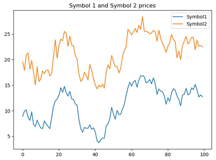
7. We build the Symbol2 prices based on the behavior of the Symbol1 prices, as shown in the code. In addition to copying the behavior of Symbol1, we will add noises. The noise is a random value following a normal distribution. The introduction of this noise is designed to mimic market fluctuations. It changes the spread value between the two symbol prices:

# Create a series for Symbol2 prices
 # We will copy the Symbol1 behavior
 noise = np.random.normal(0, 1, 100)
 Symbol2_prices = Symbol1_prices + 10 + noise
 Symbol2_prices.name = 'Symbol2'
 plt.title("Symbol 1 and Symbol 2 prices")
 Symbol1_prices.plot()
 Symbol2_prices.plot()
 plt.show()

This code will return the following output. The plot shows the evolution of the price of Symbol 1 and Symbol 2:

8. In the code, we will check the cointegration between the two symbols by using the coint function. This takes two lists/series of values and performs a test to check whether the two series are co-integrated:

score, pvalue, _ = coint(Symbol1_prices, Symbol2_prices)

In the code, pvalue contains the p-score. Its value is 10-13, which means that we can reject the null hypothesis. Therefore, these two symbols are co-integrated.

9. We will define the zscore function. This function returns how far a piece of data is from the population mean. This will help us to choose the direction of trading. If the return value of this function is positive, this means that the symbol price is higher than the average price value. Therefore, its price is expected to go down or the paired symbol value will go up. In this case, we will want to short this symbol and long the other one. The code implements the zscore function:

 def zscore(series):
     return (series - series.mean()) / np.std(series)

10. We will use the ratio between the two symbol prices. We will need to set the threshold that defines when a given price is far off the mean price value. For that, we will need to use specific values for a given symbol. If we have many symbols we want to trade with, this will imply that this analysis be performed for all the symbols. Since we want to avoid this tedious work, we are going to normalize this study by analyzing the ratio of the two prices instead. As a result, we calculate the ratios of the Symbol 1 price against the Symbol 2 price. Let's have a look at the code:

 ratios = Symbol1_prices / Symbol2_prices
 ratios.plot()

This code will return the following output. In the diagram, we show the variation in the ratio between symbol 1 and symbol 2 prices:

11. Let's draw the chart showing when we will place orders with the following code:

 train = ratios[:75]
 test = ratios[75:]
 
 plt.axhline(ratios.mean())
 plt.legend([' Ratio'])
 plt.show()
 
 zscore(ratios).plot()
 plt.axhline(zscore(ratios).mean(),color="black")
 plt.axhline(1.0, color="red")
 plt.axhline(-1.0, color="green")
 plt.show()

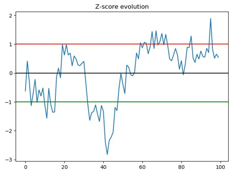
This code will return the following output. The curve demonstrates the following:

• The Z-score evolution with horizontal lines at -1 (green), +1 (red), and the average of Z-score (black).
• The average of Z-score is 0.
• When the Z-score reaches -1 or +1, we will use this event as a trading signal. The values +1 and -1 are arbitrary values.
• It should be set depending on the study we will run in order to create this trading strategy:

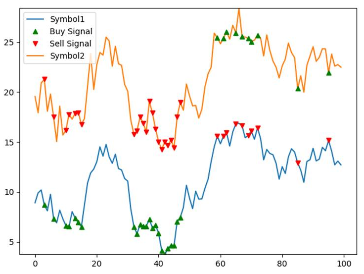
12. Every time the Z-score reaches one of the thresholds, we have a trading signal. As shown in the code, we will present a graph, each time we go long for Symbol 1 with a green marker, and each time we go short with a red marker:

 ratios.plot()
 buy = ratios.copy()
 sell = ratios.copy()
 buy[zscore(ratios)>-1] = 0
 sell[zscore(ratios)<1] = 0
 buy.plot(color="g", linestyle="None", marker="^")
 sell.plot(color="r", linestyle="None", marker="v")
 x1,x2,y1,y2 = plt.axis()
 plt.axis((x1,x2,ratios.min(),ratios.max()))
 plt.legend(["Ratio", "Buy Signal", "Sell Signal"])
 plt.show()

This code will return the following output. Let's have a look at the plot:

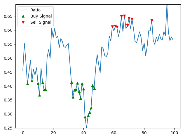
In this example, going long for Symbol 1 means that we will send a buy order for Symbol 1, while sending a sell order for Symbol 2 concurrently.

13. Next, we will write the following code, which represents the buy and sell order for each symbol:

Symbol1_prices.plot()
 symbol1_buy[zscore(ratios)>-1] = 0
 symbol1_sell[zscore(ratios)<1] = 0
 symbol1_buy.plot(color="g", linestyle="None", marker="^")
 symbol1_sell.plot(color="r", linestyle="None", marker="v")
 
 Symbol2_prices.plot()
 symbol2_buy[zscore(ratios)<1] = 0
 symbol2_sell[zscore(ratios)>-1] = 0
 symbol2_buy.plot(color="g", linestyle="None", marker="^")
 symbol2_sell.plot(color="r", linestyle="None", marker="v")
 
 
 x1,x2,y1,y2 = plt.axis()
 plt.axis((x1,x2,Symbol1_prices.min(),Symbol2_prices.max()))
 plt.legend(["Symbol1", "Buy Signal", "Sell Signal","Symbol2"])     plt.show()

The following chart shows the buy and sell orders for this strategy. We see that the orders will be placed only when zscore is higher or lower than +/-1:

Following the analysis that provided us with an understanding of the pairs that are co-integrated, we observed that the following pairs demonstrated similar behavior:

• ADBE, MSFT
• JNPR, LUV
• JNPR, MSFT
• JNPR, QCOM
• JNPR, SKYW
• JNPR, SPY

14. We will use MSFT and JNPR to implement the strategy based on real symbols. We will replace the code to build Symbol 1 and Symbol 2 with the following code. The following code will get the real prices for MSFT and JNPR:

 Symbol1_prices = data['Adj Close']['MSFT']
 Symbol1_prices.plot(figsize=(15,7))
 plt.show()
 Symbol2_prices = data['Adj Close']['JNPR']
 Symbol2_prices.name = 'JNPR'
 plt.title("MSFT and JNPR prices")
 Symbol1_prices.plot()
 Symbol2_prices.plot()
 plt.legend()
 plt.show()

This code will return the following plots as output. Let's have a look at them:

The following screenshot shows the MSFT and JNPR prices. We observe similarities of movement between the two symbols:

When running the code that we ran previously for Symbol 1 and Symbol 2 by getting the actual prices from JNPR and MSFT, we will obtain the following curves:

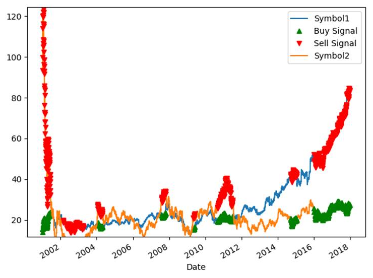
This chart reveals a large quantity of orders. The pair correlation strategy without limitation sends too many orders. We can limit the number of orders in the same way we did previously:

• Limiting positions
• Limiting the number of orders
• Setting a higher Z-score threshold

In this section, we focused on when to enter a position, but we have not addressed when to exit a position. While the Z-score value is above or below the threshold limits (in this example, -1 or +1), a Z-score value within the range between the threshold limits denotes an improbable change of spread between the two symbol prices. Therefore, when this value is within this limit, this can be regarded as an exit signal.

In the following diagram, we illustrate when we should exit a position:

In this example, the following applies:

• When the Z-score is lower than -1, we short sell Symbol 1 for $3 and we buy it for $4, while, when the Z-score is in the range [-1,+1], we exit the position by buying Symbol 2 for $1 and selling it for $3.
• If we just get 1 share of the two symbols, the profit of this trade will be ($3-$4)+($3-$1)=$1.

15. We will create a data frame, pair_correlation_trading_strategy, in the code. This contains information relating to orders and position and we will use this data frame to calculate the performance of this pair correlation trading strategy:

pair_correlation_trading_strategy = pd.DataFrame(index=Symbol1_prices.index)
 pair_correlation_trading_strategy['symbol1_price']=Symbol1_prices
 pair_correlation_trading_strategy['symbol1_buy']=np.zeros(len(Symbol1_prices))
 pair_correlation_trading_strategy['symbol1_sell']=np.zeros(len(Symbol1_prices))
 pair_correlation_trading_strategy['symbol2_buy']=np.zeros(len(Symbol1_prices))
 pair_correlation_trading_strategy['symbol2_sell']=np.zeros(len(Symbol1_prices))

16. We will limit the number of orders by reducing the position to one share. This can be a long or short position. For a given symbol, when we have a long position, a sell order is the only one that is allowed. When we have a short position, a buy order is the only one that is allowed. When we have no position, we can either go long (by buying) or go short (by selling). We will store the price we use to send the orders. For the paired symbol, we will do the opposite. When we sell Symbol 1, we will buy Symbol 2, and vice versa:

 position=0
 for i in range(len(Symbol1_prices)):
     s1price=Symbol1_prices[i]
     s2price=Symbol2_prices[i]
     if not position and symbol1_buy[i]!=0:
         pair_correlation_trading_strategy['symbol1_buy'][i]=s1price
         pair_correlation_trading_strategy['symbol2_sell'][i] = s2price
         position=1
     elif not position and symbol1_sell[i]!=0:
         pair_correlation_trading_strategy['symbol1_sell'][i] = s1price
         pair_correlation_trading_strategy['symbol2_buy'][i] = s2price
         position = -1
     elif position==-1 and (symbol1_sell[i]==0 or i==len(Symbol1_prices)-1):
         pair_correlation_trading_strategy['symbol1_buy'][i] = s1price
         pair_correlation_trading_strategy['symbol2_sell'][i] = s2price
         position = 0
     elif position==1 and (symbol1_buy[i] == 0 or i==len(Symbol1_prices)-1):
         pair_correlation_trading_strategy['symbol1_sell'][i] = s1price
         pair_correlation_trading_strategy['symbol2_buy'][i] = s2price
         position = 0

This code will return the following output. The plot shows the decrease in the number of orders. We will now calculate the profit and loss generated by this strategy:

17. We will now write the code that calculates the profit and loss of the pair correlation strategy. We make a subtraction between the vectors containing the Symbol 1 and Symbol 2 prices. We will then add these positions to create a representation of the profit and loss:

pair_correlation_trading_strategy['symbol1_position']=
 pair_correlation_trading_strategy['symbol1_buy']-pair_correlation_trading_strategy['symbol1_sell']
 
 pair_correlation_trading_strategy['symbol2_position']=
 pair_correlation_trading_strategy['symbol2_buy']-pair_correlation_trading_strategy['symbol2_sell']
 
 pair_correlation_trading_strategy['symbol1_position'].cumsum().plot() # Calculate Symbol 1 P&L
 pair_correlation_trading_strategy['symbol2_position'].cumsum().plot() # Calculate Symbol 2 P&L
 
 pair_correlation_trading_strategy['total_position']=
 pair_correlation_trading_strategy['symbol1_position']+pair_correlation_trading_strategy['symbol2_position'] # Calculate total P&L
 pair_correlation_trading_strategy['total_position'].cumsum().plot()

This code will return the following output. In the plot, the blue line represents the profit and loss for Symbol 1, and the orange line represents the profit and loss for Symbol 2. The green line represents the total profit and loss:

Until this part, we traded only one share. In regular trading, we will trade hundreds/thousands of shares. Let's analyze what can happen when we use a pair-correlation trading strategy.

Suppose we have a pair of two symbols (Symbol 1 and Symbol 2). Let's assume that the Symbol 1 price is $100 and the Symbol 2 price is $10. If we trade a given fixed amount of shares of Symbol 1 and Symbol 2, we can use 100 shares. If we have a long signal for Symbol 1, we will buy Symbol 1 for $100. The notional position will be 100 x $100 = $10,000. Since it is a long signal for Symbol 1, it is a short signal for Symbol 2. We will have a Symbol 2 notional position of 100 x $10 = $1,000. We will have a delta of $9,000 between these two positions.

By having a large price differential, this places more emphasis on the symbol with the higher price. So it means when that symbol leads the return. Additionally, when we trade and invest money on the market, we should hedge positions against market moves. For example, if we invest in an overall long position by buying many symbols, we think that these symbols will outperform the market. Suppose the whole market is depreciating, but these symbols are indeed outperforming the other ones. If we want to sell them, we will certainly lose money since the market will collapse. For that, we usually hedge our positions by investing in something that will move on the opposite side of our positions. In the example of a pair trading correlation, we should aim to have a neutral position by investing the same notional in Symbol 1 and in Symbol 2. By taking the example of having a Symbol 1 price that is markedly different to the Symbol 2 price, we cannot use the hedge of Symbol 2 if we invest the same number of shares as we invest in Symbol 1.

Because we don't want to be in either of the two situations described earlier, we are going to invest the same notional in Symbol 1 and Symbol 2. Let's say we want to buy 100 shares of Symbol 1. The notional position we will have is 100 x $100 = $10,000. To get the same equivalent of notional position for Symbol 2, we will need to get $10,000 / $10 = 1,000 shares. If we get 100 shares of Symbol 1 and 1,000 shares of Symbol 2, we will have a neutral position for this investment, and we will not give more importance to Symbol 1 over Symbol 2.

Now, let's suppose the price of symbol 2 is $3 instead of being $10. When dividing $10,000 / $3 = 3,333 + 1/3. This means we will send an order for 3,333 shares, which means that we will have a Symbol 1 position of $10,000 and a Symbol 2 position of 3,333 x $3 = $9,999, resulting in a delta of $1. Now suppose that the traded amount, instead of being $10,000, was $10,000,000. This will result in a delta of $1,000. Because we need to remove the decimal part when buying stocks, this delta will appear for any symbols. If we trade around 200 pairs of symbols, we may have $200,000 (200 x $1,000) of position that is not hedged. We will be exposed to market moves. Therefore, if the market goes down, we may lose out on this $200,000. That's why it will be important to hedge with a financial instrument going in the opposite direction from this $200,000 position. If we have positions with many symbols, resulting in having a residual of $200,000 of a long position that is not covered, we will get a short position of the ETF SPY behaving in the same way as the market moves.

18. We replace s1prices with s1positions from the earlier code by taking into account the number of shares we want to allocate for the trading of this pair:

pair_correlation_trading_strategy['symbol1_price']=Symbol1_prices
 pair_correlation_trading_strategy['symbol1_buy']=np.zeros(len(Symbol1_prices))
 pair_correlation_trading_strategy['symbol1_sell']=np.zeros(len(Symbol1_prices))
 pair_correlation_trading_strategy['symbol2_buy']=np.zeros(len(Symbol1_prices))
 pair_correlation_trading_strategy['symbol2_sell']=np.zeros(len(Symbol1_prices))
 pair_correlation_trading_strategy['delta']=np.zeros(len(Symbol1_prices)) 
 position=0
 s1_shares = 1000000
 for i in range(len(Symbol1_prices)):
     s1positions= Symbol1_prices[i] * s1_shares
     s2positions= Symbol2_prices[i] * int(s1positions/Symbol2_prices[i])
     delta_position=s1positions-s2positions
     if not position and symbol1_buy[i]!=0:
         pair_correlation_trading_strategy['symbol1_buy'][i]=s1positions
         pair_correlation_trading_strategy['symbol2_sell'][i] = s2positions
         pair_correlation_trading_strategy['delta'][i]=delta_position
         position=1
     elif not position and symbol1_sell[i]!=0:
         pair_correlation_trading_strategy['symbol1_sell'][i] = s1positions
         pair_correlation_trading_strategy['symbol2_buy'][i] = s2positions
         pair_correlation_trading_strategy['delta'][i] = delta_position
         position = -1
     elif position==-1 and (symbol1_sell[i]==0 or i==len(Symbol1_prices)-1):
         pair_correlation_trading_strategy['symbol1_buy'][i] = s1positions
         pair_correlation_trading_strategy['symbol2_sell'][i] = s2positions
         position = 0
     elif position==1 and (symbol1_buy[i] == 0 or i==len(Symbol1_prices)-1):
         pair_correlation_trading_strategy['symbol1_sell'][i] = s1positions
         pair_correlation_trading_strategy['symbol2_buy'][i] = s2positions
         position = 0

This code will return the following output. This graph represent the positions of Symbol 1 and Symbol 2 and the total profit and loss of this pair correlation trading strategy:

The code displays the delta position. The maximum amount is $25. Because this amount is too low, we don't need to hedge this delta position:

pair_correlation_trading_strategy['delta'].plot()
 plt.title("Delta Position")
 plt.show()

This section concludes the implementation of a trading strategy that is based on the correlation/cointegration with another financial product.