Given observations of the target variables, rows of features values, and each row of dimension , OLS seeks to find the weights of dimension that minimize the residual sum of squares of differences between the target variable and the predicted variable predicted by linear approximation:

• , which is the best fit for the equation , where is the  matrix of feature values, is the matrix/vector of weights/coefficients assigned to each of the  feature values, and  is the matrix/vector of the target variable observation on our training dataset.

             Here is an example of the matrix operations involved for  and :

• Intuitively, it is very easy to understand OLS with a single feature variable and a single target variable by visualizing it as trying to draw a line that has the best fit.
• OLS is just a generalization of this simple idea in much higher dimensions, where is tens of thousands of observations, and is thousands of features values.
• The typical setup in is much larger than (many more observations in comparison to the number of feature values), otherwise the solution is not guaranteed to be unique.
• There are closed form solutions to this problem where  but, in practice, these are better implemented by iterative solutions, but we'll skip the details of all of that for now.
• The reason why we prefer to minimize the sum of the squares of the error terms is so that massive outliers are penalized more harshly and don't end up throwing off the entire fit.

There are many underlying assumptions for OLS in addition to the assumption that the target variable is a linear combination of the feature values, such as the independence of feature values themselves, and normally distributed error terms. The following diagram is a very simple example showing a relatively close linear relationship between two arbitrary variables. Note that it is not a perfect linear relationship, in other words, not all data points lie perfectly on the line and we have left out the X and Y labels because these can be any arbitrary variables. The point here is to demonstrate an example of what a linear relationship visualization looks like. Let's have a look at the following diagram:

1. Let's start by loading up Google data in the code, using the same method that we introduced in the previous section:

goog_data = load_financial_data(
    start_date='2001-01-01',
    end_date='2018-01-01',
    output_file='goog_data_large.pkl')

2. Now, we create and populate the target variable vector, Y, for regression in the following code. Remember that what we are trying to predict in regression is magnitude and the direction of the price change from one day to the next:

goog_data, X, Y = create_regression_trading_condition(goog_data)

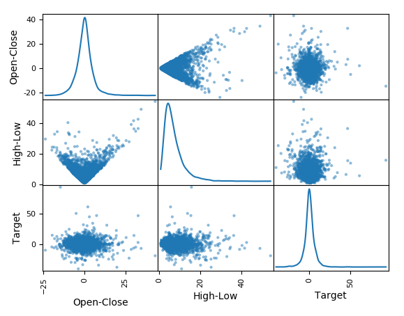
3. With the help of the code, let's quickly create a scatter plot for the two features we have: High-Low price of the day and Open-Close price of the day against the target variable, which is Price-Of-Next-Day - Price-Of-Today (future price):

pd.plotting.scatter_matrix(goog_data[['Open-Close', 'High-Low', 'Target']], grid=True, diagonal='kde')

This code will return the following output. Let's have a look at the plot:

4. Finally, as shown in the code, let's split 80% of the available data into the training feature value and target variable set (X_train, Y_train), and the remaining 20% of the dataset into the out-sample testing feature value and target variable set (X_test, Y_test):

X_train,X_test,Y_train,Y_test=create_train_split_group(X,Y,split_ratio=0.8)

5. Now, let's fit the OLS model as shown here and observe the model we obtain:

from sklearn import linear_model
ols = linear_model.LinearRegression()
ols.fit(X_train, Y_train)

6. The coefficients are the optimal weights assigned to the two features by the fit method. We will print the coefficients as shown in the code:

print('Coefficients: 
', ols.coef_)

This code will return the following output. Let's have a look at the coefficients:

Coefficients:
[[ 0.02406874 -0.05747032]]

7. The next block of code quantifies two very common metrics that test goodness of fit for the linear model we just built. Goodness of fit means how well a given model fits the data points observed in training and testing data. A good model is able to closely fit most of the data points and errors/deviations between observed and predicted values are very low. Two of the most popular metrics for linear regression models are mean_squared_error , which is what we explored as our objective to minimize when we introduced OLS, and R-squared (), which is another very popular metric that measures how well the fitted model predicts the target variable when compared to a baseline model whose prediction output is always the mean of the target variable based on training data, that is, . We will skip the exact formulas for computing  but, intuitively, the closer the  value to 1, the better the fit, and the closer the  value to 0, the worse the fit. Negative  values mean that the model fits worse than the baseline model. Models with negative  values usually indicate issues in the training data or process and cannot be used:

from sklearn.metrics import mean_squared_error, r2_score

# The mean squared error
print("Mean squared error: %.2f"
      % mean_squared_error(Y_train, ols.predict(X_train)))

# Explained variance score: 1 is perfect prediction
print('Variance score: %.2f' % r2_score(Y_train, ols.predict(X_train)))

# The mean squared error
print("Mean squared error: %.2f"
      % mean_squared_error(Y_test, ols.predict(X_test)))

# Explained variance score: 1 is perfect prediction
print('Variance score: %.2f' % r2_score(Y_test, ols.predict(X_test)))

This code will return the following output:

Mean squared error: 27.36
Variance score: 0.00
Mean squared error: 103.50
Variance score: -0.01

8. Finally, as shown in the code, let's use it to predict prices and calculate strategy returns:

goog_data['Predicted_Signal'] = ols.predict(X)
goog_data['GOOG_Returns'] = np.log(goog_data['Close'] / goog_data['Close'].shift(1))

def calculate_return(df, split_value, symbol):
    cum_goog_return = df[split_value:]['%s_Returns' % symbol].cumsum() * 100
    df['Strategy_Returns'] = df['%s_Returns' % symbol] * df['Predicted_Signal'].shift(1)
    return cum_goog_return

def calculate_strategy_return(df, split_value, symbol):
    cum_strategy_return = df[split_value:]['Strategy_Returns'].cumsum() * 100
    return cum_strategy_return

cum_goog_return = calculate_return(goog_data, split_value=len(X_train), symbol='GOOG')
cum_strategy_return = calculate_strategy_return(goog_data, split_value=len(X_train), symbol='GOOG')

def plot_chart(cum_symbol_return, cum_strategy_return, symbol):
    plt.figure(figsize=(10, 5))
    plt.plot(cum_symbol_return, label='%s Returns' % symbol)
    plt.plot(cum_strategy_return, label='Strategy Returns')
    plt.legend()

plot_chart(cum_goog_return, cum_strategy_return, symbol='GOOG')

def sharpe_ratio(symbol_returns, strategy_returns):
    strategy_std = strategy_returns.std()
    sharpe = (strategy_returns - symbol_returns) / strategy_std
    return sharpe.mean()

print(sharpe_ratio(cum_strategy_return, cum_goog_return))

This code will return the following output:

2.083840359081768

Let's now have a look at the graphical representation that is derived from the code:

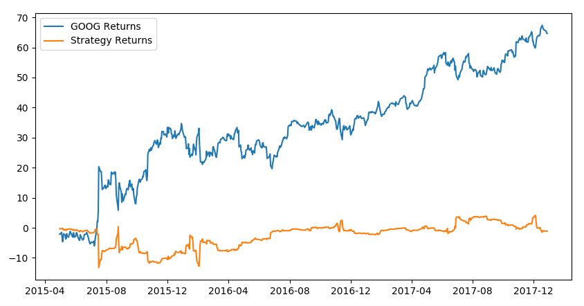
Here, we can observe that the simple linear regression model using only the two features, Open-Close and High-Low, returns positive returns. However, it does not outperform the Google stock's return because it has been increasing in value since inception. But since that cannot be known ahead of time, the linear regression model, which does not assume/expect increasing stock prices, is a good investment strategy.