Learning Objectives
By the end of this chapter, you will be able to:
- Describe the fundamental concepts of classification
- Load and preprocess data for classification
- Implement k-nearest neighbor and support vector machine classifiers
In chapter will focus on the goals of classification, and learn about k-nearest neighbors and support vector machines.
4
Introduction
In this chapter, we will learn about classifiers, especially the k-nearest neighbor classifier and support vector machines. We will use this classification to categorize data. Just as we did for regression, we will build a classifier based on training data, and test the performance of our classifier using testing data.
The Fundamentals of Classification
While regression focuses on creating a model that best fits our data to predict the future, classification is all about creating a model that separates our data into separate classes.
Assuming that you have some data belonging to separate classes, classification helps you predict the class a new data point belongs to. A classifier is a model that determines the label value belonging to any data point in the domain. Suppose you have a set of points, P = {p1, p2, p3, ..., pm}, and another set of points, Q = {q1, q2, q3, ..., qn}. You treat these points as members of different classes. For simplicity, we could imagine that P contains credit-worthy individuals, and Q contains individuals that are risky in terms of their credit repayment tendencies.
You can divide the state space so that all points in P are on one cluster of the state space, and then disjoint from the state space cluster containing all points in Q. Once you find these bounded spaces, called clusters, inside the state space, you have successfully performed clustering.
Suppose we have a point, x, that's not equal to any of the previous points. Does point x belong to cluster P or cluster Q? The answer to this question is a classification exercise, because we classify point x.
Classification is usually determined by proximity. The closer point x is to points in cluster P, the more likely it is that it belongs to cluster P . This is the idea behind nearest neighbor classification. In the case of k-nearest neighbor classification, we find the k-nearest neighbor of point x and classify it according to the maximum number of the nearest neighbors from the same class. Besides k-nearest neighbor, we will also use support vector machines for classification. In this chapter, we will be covering this credit scoring method in detail.
We could either assemble random dummy data ourselves, or we could choose to use an online dataset with hundreds of data points. To make this learning experience as realistic as possible, we will choose the latter. Let's continue with an exercise that lets us download some data that we can use for classification. A popular place for downloading machine learning datasets is https://archive.ics.uci.edu/ml/datasets.html. You can find five different datasets on credit approval. We will now load the dataset on German credit approvals, because the size of 1,000 data points is perfect for an example, and its documentation is available.
The german dataset is available in the CSV format
CSV stands for comma-separated values. A CSV file is a simple text file, where each line of the file contains a data point in your dataset. The attributes of the data point are given in a fixed order, separated by a separator character such as a comma. This character may not occur in the data, otherwise we would not know if the separator character is part of the data or serves as a separator. Although the name comma-separated values suggests that the separator character is a comma, it is not always the case. For instance, in our example, the separator character is a space. CSV files are used in many applications, including Excel. CSV is a great, lean interface between different applications.
Exercise 10: Loading Datasets
- Visit https://archive.ics.uci.edu/ml/datasets/Statlog+%28German+Credit+Data%29. The data files are located at https://archive.ics.uci.edu/ml/machine-learning-databases/statlog/german/.
Load the data from the space-separated german.data file. Make sure that you add headers to your DataFrame so that you can reference your features and labels by name instead of column number.
Save the german.data file locally. Insert header data into your CSV file.
The first few lines of the dataset are as follows:
A11 6 A34 A43 1169 A65 A75 4 A93 A101 4 A121 67 A143 A152 2 A173 1 A192 A201 1
A12 48 A32 A43 5951 A61 A73 2 A92 A101 2 A121 22 A143 A152 1 A173 1 A191 A201 2
A14 12 A34 A46 2096 A61 A74 2 A93 A101 3 A121 49 A143 A152 1 A172 2 A191 A201 1
The explanation to interpret this data is in the german.doc file, where you can see the list of attributes. These attributes are: Status of existing checking account (A11 – A14), Duration (numeric, number of months), Credit history (A30 - A34), Purpose of credit (A40 – A410), Credit amount (numeric), Savings account/bonds (A61 – A65), Present employment since (A71 – A75), Disposable income percent rate (numeric), Personal status and sex (A91 – A95), Other debtors and guarantors (A101 – A103), Present residence since (numeric), Property (A121 – A124), Age (numeric, years), Other installment plans (A141 – A143), Housing (A151 – A153), Number of existing credits at this bank, Job (A171 – A174), Number of people being liable to provide maintenance for (numeric) Telephone (A191 – A192) and Foreign worker (A201 – A202).
The result of classification would be as follows: 1 means good debtor, while 2 means bad debtor.
Our task is to determine how to separate the state space of twenty input variables into two clusters: good debtors and bad debtors.
- We will use the pandas library to load the data. Before loading the data, though, I suggest adding a header to the german.data file. Insert the following header line before the first line:
CheckingAccountStatus DurationMonths CreditHistory CreditPurpose CreditAmount SavingsAccount EmploymentSince DisposableIncomePercent PersonalStatusSex OtherDebtors PresentResidenceMonths Property Age OtherInstallmentPlans Housing NumberOfExistingCreditsInBank Job LiabilityNumberOfPeople Phone ForeignWorker CreditScore
Notice that the preceding header is just one line, which means that there is no newline character until the end of the 21st label, CreditScore.
Note
The header is of help because pandas can interpret the first line as the column name. In fact, this is the default behavior of the read_csv method of pandas. The first line of the .csv file is going to be the header, and the rest of the lines are the actual data.
Let's import the CSV data using the pandas.read_csv method:
import pandas
data_frame = pandas.read_csv('german.data', sep=' ')
- The first argument of read_csv is the file path. If you saved it to the E drive of your Windows PC, for instance, then you can also write an absolute path there: e:german.data.

Figure 4.1: Table displaying list of attributes in respective cells
Let's see the format of the data. The data_frame.head() call prints the first five rows of the CSV file, structured by the pandas DataFrame:
data_frame.head()
The output will be as follows:
CheckingAccountStatus DurationMonths CreditHistory CreditPurpose
0 A11 6 A34 A43
..
4 A11 24 A33 A40
CreditAmount SavingsAccount EmploymentSince DisposableIncomePercent
0 1169 A65 A75 4
..
4 4870 A61 A73 3
PersonalStatusSex OtherDebtors ... Property Age
0 A93 A101 ... A121 67
..
4 A93 A101 ... A124 53
OtherInstallmentPlans Housing NumberOfExistingCreditsInBank Job
0 A143 A152 2 A173
..
4 A143 A153 2 A173
LiabilityNumberOfPeople Phone ForeignWorker CreditScore
0 1 A192 A201 1
..
4 2 A191 A201 2
[5 rows x 21 columns]
We have successfully loaded the data into the DataFrame.
Data Preprocessing
Before building a classifier, we are better off formatting our data so that we can keep relevant data in the most suitable format for classification, and removing all data that we are not interested in.
1. Replacing or dropping values
For instance, if there are N/A (or NA) values in the dataset, we may be better off substituting these values with a numeric value we can handle. NA stands for Not Available. We may choose to ignore rows with NA values or replace them with an outlier value. An outlier value is a value such as -1,000,000 that clearly stands out from regular values in the dataset. The replace method of a DataFrame does this type of replacement. The replacement of NA values with an outlier looks as follows:
data_frame.replace('NA', -1000000, inplace=True)
The replace method changes all NA values to numeric values.
This numeric value should be far from any reasonable values in the DataFrame. Minus one million is recognized by the classifier as an exception, assuming that only positive values are there.
The alternative to replacing unavailable data with extreme values is dropping the rows that have unavailable data:
data_frame.dropna(0, inplace=True)
The first argument specifies that we drop rows, not columns. The second argument specifies that we perform the drop operation, without cloning the DataFrame. Dropping the NA values is less desirable, as you often lose a reasonable chunk of your dataset.
2. Dropping columns
If there is a column we do not want to include in the classification, we are better off dropping it. Otherwise, the classifier may detect false patterns in places where there is absolutely no correlation. For instance, your phone number itself is very unlikely to correlate with your credit score. It is a 9 to 12-digit number that may very easily feed the classifier with a lot of noise. So we drop the phone column.
data_frame.drop(['Phone'], 1, inplace=True)
The second argument indicates that we drop columns, not rows. The first argument is an enumeration of the columns we would like to drop. The inplace argument is so that the call modifies the original DataFrame.
3. Transforming data
Oftentimes, the data format we are working with is not always optimal for the classification process. We may want to transform our data into a different format for multiple reasons, such as the following:
- To highlight aspects of data we are interested in (for example, Minmax scaling or normalization)
- To drop aspects of data we are not interested in (for example, Binarization)
- Label encoding
Minmax scaling can be performed by the MinMaxScaler method of the scikit preprocessing utility:
from sklearn import preprocessing
data = np.array([
[19, 65],
[4, 52],
[2, 33]
])
preprocessing.MinMaxScaler(feature_range=(0,1)).fit_transform(data)
The output is as follows:
array([[1. , 1. ],
[0.11764706, 0.59375 ],
[0. , 0. ]])
MinMaxScaler scales each column in the data so that the lowest number in the column becomes 0, the highest number becomes 1, and all of the values in between are proportionally scaled between zero and one.
Binarization transforms data into ones and zeros based on a condition:
preprocessing.Binarizer(threshold=10).transform(data)
array([[1, 1],
[0, 1],
[0, 1]])
Label encoding is important for preparing your features for scikit-learn to process. While some of your features are string labels, scikit-learn expects this data to be numbers.
This is where the preprocessing library of scikit-learn comes into play.
Note
You might have noticed that in the credit scoring example, there were two data files. One contained labels in string form, and the other in integer form. I asked you to load the data with string labels on purpose so that you got some experience of how to preprocess data properly with the label encoder.
Label encoding is not rocket science. It creates a mapping between string labels and numeric values so that we can supply numbers to scikit-learn:
from sklearn import preprocessing
labels = ['Monday', 'Tuesday', 'Wednesday', 'Thursday', 'Friday']
label_encoder = preprocessing.LabelEncoder()
label_encoder.fit(labels)
Let's enumerate the encoding:
[x for x in enumerate(label_encoder.classes_)]
The output will be as follows:
[(0, 'Friday'),
(1, 'Monday'),
(2, 'Thursday'),
(3, 'Tuesday'),
(4, 'Wednesday')]
We can use the encoder to transform values:
encoded_values = label_encoder.transform(['Wednesday', 'Friday'])
The output will be as follows:
array([4, 0], dtype=int64)
The inverse transformation that transforms encoded values back to labels is performed by the inverse_transform function:
label_encoder.inverse_transform([0, 4])
The output will be as follows:
array(['Wednesday', 'Friday'], dtype='<U9')
Exercise 11: Pre-Processing Data
In this exercise, we will use a dataset with pandas.
- Load the CSV data of the 2017-2018 January kickstarter projects from https://github.com/TrainingByPackt/Artificial-Intelligence-and-Machine-Learning-Fundamentals/blob/master/Lesson04/Exercise%2011%20Pre-processing%20Data/ks-projects-201801.csv and apply the preprocessing steps on the loaded data.
Note
Note that you need a working internet connection to complete this exercise.
- If you open the file, you will see that you don't have to bother adding a header, because it is included in the CSV file:
ID,name,category,main_category,currency,deadline,goal,launched,pledged,state,backers,country,usd pledged,usd_pledged_real,usd_goal_real
- Import the data and create a DataFrame using pandas:
import pandas
data_frame = pandas.read_csv('ks-projects-201801.csv', sep=',')
data_frame.head()
- The previous command prints the first five entries belonging to the dataset. We can see the name and format of each column. Now that we have the data, it's time to perform some preprocessing steps.
- Suppose you have some NA or N/A values in the dataset. You can replace them with the following replace operations:
data_frame.replace('NA', -1000000, inplace=True)
data_frame.replace('N/A', -1000000, inplace=True)
- When performing classification or regression, keeping the ID column is just asking for trouble. In most cases, the ID does not correlate with the end result. Therefore, it makes sense to drop the ID column:
data_frame.drop(['ID'], 1, inplace=True)
- Suppose we are only interested in whether the projects had backers or not. This is a perfect case for binarization:
from sklearn import preprocessing
preprocessing.Binarizer(threshold=1).transform([data_frame['backers']])
- The output will be as follows:
array([[0, 1, 1, ..., 0, 1, 1]], dtype=int64)
Note
We are discarding the resulting binary array. To make use of the binary data, we would have to replace the backers column with it. We will omit this step for simplicity.
- Let's encode the labels so that they become numeric values that can be interpreted by the classifier:
labels = ['AUD', 'CAD', 'CHF', 'DKK', 'EUR', 'GBP', 'HKD', 'JPY', 'MXN', 'NOK', 'NZD', 'SEK', 'SGD', 'USD']
label_encoder = preprocessing.LabelEncoder()
label_encoder.fit(labels)
label_encoder.transform(data_frame['currency'])
- The output will be as follows:
array([ 5, 13, 13, ..., 13, 13, 13], dtype=int64)
You have to know about all possible labels that can occur in your file. The documentation is responsible for providing you with the available options. In the unlikely case that the documentation is not available for you, you have to reverse engineer the possible values from the file.
Once the encoded array is returned, the same problem holds as in the previous point: we have to make use of these values by replacing the currency column of the DataFrame with these new values.
Minmax Scaling of the Goal Column
When Minmax scaling was introduced, you saw that instead of scaling the values of each vector in a matrix, the values of each coordinate in each vector were scaled together. This is how the matrix structure describes a dataset. One vector contains all attributes of a data point. When scaling just one attribute, we have to transpose the column we wish to scale.
You learned about the transpose operation of NumPy in Chapter 1, Principles of Artificial Intelligence:
import numpy as np
values_to_scale = np.mat([data_frame['goal']]).transpose()
Then, we have to apply the MinMaxScaler to scale the transposed values. To get the results in one array, we can transpose the results back to their original form:
preprocessing
.MinMaxScaler(feature_range=(0,1))
.fit_transform(values_to_scale)
.transpose()
The output is as follows:
array([[9.999900e-06, 2.999999e-04, 4.499999e-04, ..., 1.499999e-04, 1.499999e-04, 1.999990e-05]])
The values look weird because there were some high goals on Kickstarter, possibly using seven figure values. Instead of linear Minmax scaling, it is also possible to use the magnitude and scale logarithmically, counting how many digits the goal price has. This is another transformation that could make sense for reducing the complexity of the classification exercise.
As always, you have to place the results in the corresponding column of the DataFrame to make use of the transformed values.
We will stop preprocessing here. Hopefully, the usage of these different methods is now clear, and you will have a strong command of using these preprocessing methods in the future.
Identifying Features and Labels
Similar to regression, in classification, we must also separate our features and labels. Continuing from the original example, our features are all columns, except the last one, which contains the result of the credit scoring. Our only label is the credit scoring column.
We will use NumPy arrays to store our features and labels:
import numpy as np
features = np.array(data_frame.drop(['CreditScore'], 1))
label = np.array(data_frame['CreditScore'])
Now that we are ready with our features and labels, we can use this data for cross-validation.
Cross-Validation with scikit-learn
Another pertinent point about regression is that we can use cross-validation to train and test our model. This process is exactly the same as in the case of regression problems:
from sklearn import model_selection
features_train, features_test, label_train, label_test =
model_selection.train_test_split(
features,
label,
test_size=0.1
)
The train_test_split method shuffles and then splits our features and labels into a training dataset and a testing dataset. We can specify the size of the testing dataset as a number between 0 and 1. A test_size of 0.1 means that 10% of the data will go into the testing dataset.
Activity 7: Preparing Credit Data for Classification
In this section, we will discuss how to prepare data for a classifier. We will be using german.data from https://archive.ics.uci.edu/ml/machine-learning-databases/statlog/german/ as an example and will prepare the data for training and testing a classifier. Make sure that all of your labels are numeric, and that the values are prepared for classification. Use 80% of the data points as training data:
- Save german.data from https://archive.ics.uci.edu/ml/machine-learning-databases/statlog/german/ and open it in a text editor such as Sublime Text or Atom. Add the header row to it.
- Import the data file using pandas and replace the NA values with an outlier value.
- Perform label encoding. Transform all of the labels in the data frame into integers.
- Separate features from labels. We can apply the same method as the one we saw in the theory section.
- Perform scaling of the training and testing data together. Use MinMaxScaler from Scikit's Preprocessing library.
- The final step is cross-validation. Shuffle our data and use 80% of all data for training and 20% for testing.
Note
The solution to this activity is available at page 276.
The k-nearest neighbor Classifier
We will continue from where we left off in the first topic. We have training and testing data, and it is now time to prepare our classifier to perform k-nearest neighbor classification. After introducing the K-Nearest Neighbor algorithm, we will use scikit-learn to perform classification.
Introducing the K-Nearest Neighbor Algorithm
The goal of classification algorithms is to divide data so that we can determine which data points belong to which region. Suppose that a set of classified points is given. Our task is to determine which class a new data point belongs to.
The k-nearest neighbor classifier receives classes of data points with given feature and label values. The goal of the algorithm is to classify data points. These data points contain feature coordinates, and the objective of the classification is to determine the label values. Classification is based on proximity. Proximity is defined as a Euclidean distance. Point A is closer to point B than to point C if the Euclidean distance between A and B is shorter than the Euclidean distance between A and C.
The k-nearest neighbor classifier gets the k-nearest neighbors of a data point. The label belonging to point A is the most frequently occurring label value among the k-nearest neighbors of point A. Determining the value of K is a non-obvious task. Obviously, if there are two groups, such as credit-worthy and not credit-worthy, we need K to be 3 or greater, because otherwise, with K=2, we could easily have a tie between the number of neighbors. In general, though, the value of K does not depend on the number of groups or the number of features.
A special case of k-nearest neighbors is when K=1. In this case, the classification boils down to finding the nearest neighbor of a point. K=1 most often gives us significantly worse results than K=3 or greater.
Distance Functions
Many distance metrics could work with the k-nearest neighbor algorithm. We will now calculate the Euclidean and the Manhattan distance of two data points. The Euclidean distance is a generalization of the way we calculate the distance of two points in the plane or in a three-dimensional space.
The distance between points A = (a1, a2, …, an) and B=(b1, b2, …, bn) is the length of the line segment connecting these two points:

Figure 4.2: Distance between points A and B
Technically, we don't need to calculate the square root when we are just looking for the nearest neighbors, because the square root is a monotone function.
As we will use the Euclidean distance in this book, let's see how to calculate the distance of multiple points using one scikit-learn function call. We have to import euclidean_distances from sklearn.metrics.pairwise. This function accepts two sets of points and returns a matrix that contains the pairwise distance of each point from the first and the second sets of points:
from sklearn.metrics.pairwise import euclidean_distances
points = [[2,3], [3,7], [1,6]]
euclidean_distances([[4,4]], points)
The output is as follows:
array([[2.23606798, 3.16227766, 3.60555128]])
For instance, the distance of (4,4) and (3,7) is approximately 3.162.
We can also calculate the Euclidean distances between points in the same set:
euclidean_distances(points)
array([[0. , 4.12310563, 3.16227766],
[4.12310563, 0. , 2.23606798],
[3.16227766, 2.23606798, 0. ]])
The Manhattan/Hamming Distance
The Hamming and Manhattan distances represent the same formula.
The Manhattan distance relies on calculating the absolute value of the difference of the coordinates of the data points:

Figure 4.3: The Manhattan and Hamming Distance
The Euclidean distance is a more accurate generalization of distance, while the Manhattan distance is slightly easier to calculate.
Exercise 12: Illustrating the K-nearest Neighbor Classifier Algorithm
Suppose we have a list of employee data. Our features are the numbers of hours worked per week and yearly salary. Our label indicates whether an employee has stayed with our company for more than two years. The length of stay is represented by a zero if it is less than two years, and a one in case it is greater than or equal to two years.
We would like to create a 3-nearest neighbor classifier that determines whether an employee stays with our company for at least two years.
Then, we would like to use this classifier to predict whether an employee with a request to work 32 hours a week and earning 52,000 dollars per year is going to stay with the company for two years or not.
The dataset is as follows:
employees = [
[20, 50000, 0],
[24, 45000, 0],
[32, 48000, 0],
[24, 55000, 0],
[40, 50000, 0],
[40, 62000, 1],
[40, 48000, 1],
[32, 55000, 1],
[40, 72000, 1],
[32, 60000, 1]
]
- Scale the features:
import matplotlib.pyplot as plot
from sklearn import preprocessing
import numpy as np
from sklearn.preprocessing import MinMaxScaler
scaled_employees = preprocessing.MinMaxScaler(feature_range=(0,1))
.fit_transform(employees)
The scaled result is as follows:
array([[0. , 0.18518519, 0. ],
[0.2 , 0. , 0. ],
[0.6 , 0.11111111, 0. ],
[0.2 , 0.37037037, 0. ],
[1. , 0.18518519, 0. ],
[1. , 0.62962963, 1. ],
[1. , 0.11111111, 1. ],
[0.6 , 0.37037037, 1. ],
[1. , 1. , 1. ],
[0.6 , 0.55555556, 1. ]])
It makes sense to scale our requested employee as well at this point: [32, 52000] becomes [ (32-24)/(40 - 24), (52000-45000)/(72000 - 45000)] = [0.5, 0.25925925925925924].
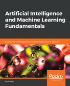
- Plot these points on a two-dimensional plane such that the first two coordinates represent a point on the plane, and the third coordinate determines the color of the point:
import matplotlib.pyplot as plot
[
plot.scatter(x[0], x[1], color = 'g' if x[2] > 0.5 else 'r')
for x in scaled_employees
] + [plot.scatter(0.5, 0.25925925925925924, color='b')]
The output is as follows:
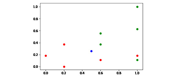
Figure 4.4: Points plotted on a two-dimensional plane
- To calculate the distance of the blue point and all the other points, we will apply the transpose function from Chapter 1, Principles of AI. If we transpose the scaledEmployee matrix, we get three arrays of ten. The feature values are in the first two arrays. We can simply use the [:2] index to keep them. Then, transposing this matrix back to its original form gives us the array of feature data points:
scaled_employee_features = scaled_employees.transpose()[:2].transpose()
scaled_employee_features
The output is as follows:
array([[0. , 0.18518519],
[0.2 , 0. ],
[0.6 , 0.11111111],
[0.2 , 0.37037037],
[1. , 0.18518519],
[1. , 0.62962963],
[1. , 0.11111111],
[0.6 , 0.37037037],
[1. , 1. ],
[0.6 , 0.55555556]])
- Calculate the Euclidean distance using:
from sklearn.metrics.pairwise import euclidean_distances
euclidean_distances(
[[0.5, 0.25925925925925924]],
scaled_employee_features
)
The output is as follows:
array([[0.50545719, 0.39650393, 0.17873968, 0.31991511, 0.50545719,
0.62223325, 0.52148622, 0.14948471, 0.89369841, 0.31271632]])
The shortest distances are as follows:
- 0.14948471 for the point [0.6, 0.37037037, 1.]
- 0.17873968 for the point [0.6, 0.11111111, 0.]
- 0.31271632 for the point [0.6, 0.55555556, 1.]
As two out of the three points have a label of 1, we found two green points and one red point. This means that our 3-nearest neighbor classifier classified the new employee as being more likely to stay for at least two years than not at all.
Note
Although, the fourth point just missed the top three by a very small margin. In fact, our algorithm would have found a tie if there were two points of a different color that had the third smallest distance from the target. In case of a race condition in distances, there could be a tie. This is an edge case, though, which should almost never occur in real-life problems.
Exercise 13: k-nearest Neighbor Classification in scikit-learn
- Split our data into four categories: training and testing, features, and labels:
from sklearn import model_selection
import pandas
import numpy as np
from sklearn import preprocessing
features_train, features_test, label_train, label_test =
model_selection.train_test_split(
scaled_features,
label,
test_size=0.2
)
- Create a K-Nearest Neighbor classifier to perform this classification:
from sklearn import neighbors
classifier = neighbors.KNeighborsClassifier()
classifier.fit(features_train, label_train)
Since we have not mentioned the value of K, the default is 5.
- Check how well our classifier performs on the test data:
classifier.score(features_test, label_test)
The output is 0.665.
You might find higher ratings with other datasets, but it is understandable that more than 20 features may easily contain some random noise that makes it difficult to classify data.
Exercise 14: Prediction with the k-nearest neighbors classifier
This code is built on the code of previous exercise.
- We'll create a data point that we will classify by taking the ith element of the ith test data point:
data_point = [None] * 20
for i in range(20):
data_point[i] = features_test[i][i]
data_point = np.array(data_point)
- We have a one-dimensional array. The classifier expects an array containing data point arrays. Therefore, we must reshape our data point into an array of data points:
data_point = data_point.reshape(1, -1)
- With this, we have created a completely random persona, and we are interested in whether they are classified as credit-worthy or not:
credit_rating = classifier.predict(data_point)
Now, we can safely use prediction to determine the credit rating of the data point:
classifier.predict(data_point)
The output is as follows:
array([1], dtype=int64)
We have successfully rated a new user based on input data.
Parameterization of the k-nearest neighbor Classifier in scikit-learn
You can access the documentation of the k-nearest neighbor classifier here: http://scikit-learn.org/stable/modules/generated/sklearn.neighbors.KNeighborsClassifier.html.
The parameterization of the classifier may fine-tune the accuracy of your classifier. Since we haven't learned all of the possible variations of k-nearest neighbor, we will concentrate on the parameters that you already understand based on this topic.
n_neighbors: This is the k value of the k-nearest neighbor algorithm. The default value is 5.
metric: When creating the classifier, you will see a weird name – "Minkowski". Don't worry about this name – you have learned about the first and second order Minkowski metric already. This metric has a power parameter. For p=1, the Minkowski metric is the same as the Manhattan metric. For p=2, the Minkowski metric is the same as the Euclidean metric.
p: This is the power of the Minkowski metric. The default value is 2.
You have to specify these parameters once you create the classifier:
classifier = neighbors.KNeighborsClassifier(n_neighbors=50)
Activity 8: Increasing the Accuracy of Credit Scoring
In this section, we will learn how the parameterization of the k-nearest neighbor classifier affects the end result. The accuracy of credit scoring is currently quite low: 66.5%. Find a way to increase it by a few percentage points. To ensure that this happens correctly, you will need to have done the previous exercises.
There are many ways to complete this exercise. In this solution, I will show you one way to increase the credit score, which will be done by changing the parameterization:
- Increase the k-value of the k-nearest neighbor classifier from the default 5 to 10, 15, 25, and 50.
- Run this classifier for all four n_neighbors values and observe the results.
- Higher K values do not necessarily mean a better score. In this example, though, K=50 yielded a better result than K=5.
Note
The solution to this activity is available at page 280.
Classification with Support Vector Machines
We first used support vector machines for regression in Chapter 3, Regression. In this topic, you will find out how to use support vector machines for classification. As always, we will use scikit-learn to run our examples in practice.
What are Support Vector Machine Classifiers?
The goal of a support vector machines defined on an n-dimensional vector space is to find a surface in that n-dimensional space that separates the data points in that space into multiple classes.
In two dimensions, this surface is often a straight line. In three dimensions, the support vector machines often finds a plane. In general, the support vector machines finds a hyperplane. These surfaces are optimal in the sense that, based on the information available to the machine, it optimizes the separation of the n-dimensional spaces.
The optimal separator found by the support vector machines is called the best separating hyperplane.
A support vector machines is used to find one surface that separates two sets of data points. In other words, support vector machines are binary classifiers. This does not mean that support vector machines can only be used for binary classification. Although we were only talking about one plane, support vector machines can be used to partition a space into any number of classes by generalizing the task itself.
The separator surface is optimal in the sense that it maximizes the distance of each data point from the separator surface.
A vector is a mathematical structure defined on an n-dimensional space having a magnitude (length) and a direction. In two dimensions, you draw the vector (x, y) from the origin to the point (x, y). Based on geometry, you can calculate the length of the vector using the Pythagorean theorem, and the direction of the vector by calculating the angle between the horizontal axis and the vector.
For instance, in two dimensions, the vector (3, -4) has the following magnitude:
sqrt( 3 * 3 + 4 * 4 ) = sqrt( 25 ) = 5
And it has the following direction:
np.arctan(-4/3) / 2 / np.pi * 360 = -53.13010235415597 degrees
Understanding Support Vector Machines
Suppose that two sets of points, Red and Blue, are given. For simplicity, we can imagine a two-dimensional plane with two features: one mapped on the horizontal axis, and one on the vertical axis.
The objective of the support vector machine is to find the best separating line that separates points A, D, C, B, and H from points E, F, and G:
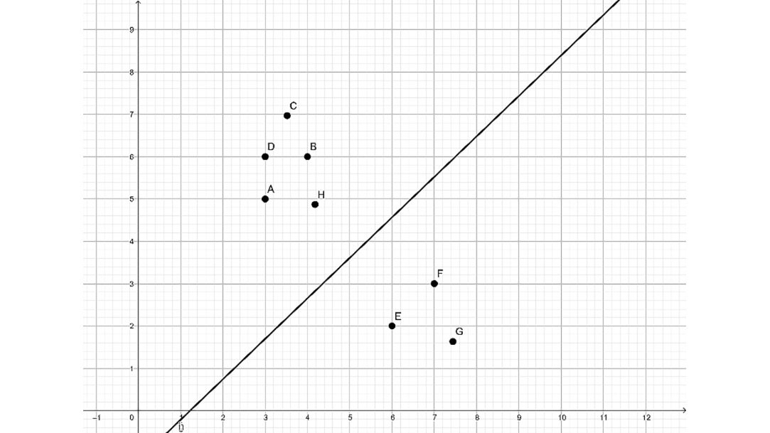
Figure 4.5: Line separating red and blue members
Separation is not always that obvious. For instance, if there is a blue point in between E, F, and G, there is no line that could separate all points without errors. If points in the blue class form a full circle around the points in the red class, there is no straight line that could separate the two sets:
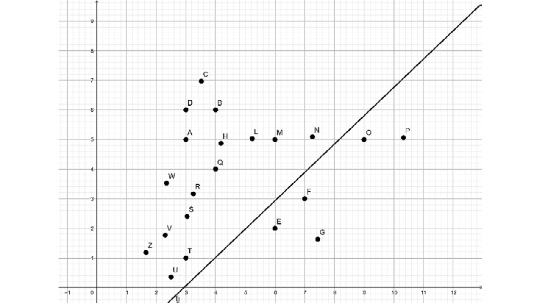
Figure 4.6: Graph with two outlier points
For instance, in the preceding graph, we tolerate two outlier points, O and P.
In the following solution, we do not tolerate outliers, and instead of a line, we create a best separating path consisting of two half lines:
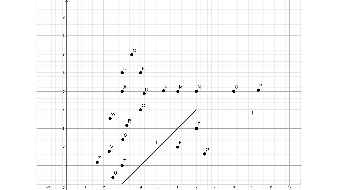
Figure 4.7: Graph removing the separation of the two outliers
A perfect separation of all data points is rarely worth the resources. Therefore, the support vector machine can be regularized to simplify and restrict the definition of the best separating shape and to allow outliers.
The regularization parameter of a support vector machine determines the rate of error to allow or forbid misclassifications.
A support vector machine has a kernel parameter. A linear kernel strictly uses a linear equation for describing the best separating hyperplane. A polynomial kernel uses a polynomial, while an exponential kernel uses an exponential expression to describe the hyperplane.
A margin is an area centered around the separator and is bounded by the points closest to the separator. A balanced margin has points from each class that are equidistant from the line.
When it comes to defining the allowed error rate of the best separating hyperplane, a gamma parameter decides whether only the points near the separator count in determining the position of the separator, or whether the points farthest from the line count, too. The higher the gamma, the lower the amount of points that influence the location of the separator.
Support Vector Machines in scikit-learn
Our entry point is the end result of previous activity. Once we have split the training and test data, we are ready to set up the classifier:
features_train, features_test, label_train, label_test = model_selection
.train_test_split(
scaled_features,
label,
test_size=0.2
)
Instead of using the K-Nearest Neighbor classifier, we will use the svm.SVC() classifier:
from sklearn import svm
classifier = svm.SVC()
classifier.fit(features_train, label_train)
# Let's can check how well our classifier performs on the
# test data:
classifier.score(features_test, label_test)
The output is 0.745.
It seems that the default support vector machine classifier of scikit-learn does a slightly better job than the k-nearest neighbor classifier.
Parameters of the scikit-learn SVM
The following are the parameters of the scikit-learn SVM:
Kernel: This is a string or callable parameter specifying the kernel used in the algorithm. The predefined kernels are linear, poly, rbf, sigmoid, and precomputed. The default value is rbf.
Degree: When using a polynomial, you can specify the degree of the polynomial. The default value is 3.
Gamma: This is the kernel coefficient for rbf, poly, and sigmoid. The default value is auto, computed as 1/number_of_features.
C: This is a floating-point number with a default of 1.0 describing the penalty parameter of the error term.
You can read about rest parameters in the reference documentation at http://scikit-learn.org/stable/modules/generated/sklearn.svm.SVC.html.
Here is an example of SVM:
classifier = svm.SVC(kernel="poly", C=2, degree=4, gamma=0.05)
Activity 9: Support Vector Machine Optimization in scikit-learn
In this section, we will discuss how to use the different parameters of a support vector machine classifier. We will be using, comparing, and contrasting the different support vector regression classifier parameters you have learned about and will find a set of parameters resulting in the highest classification data on the training and testing data that we loaded and prepared in the previous activity. To ensure that you can complete this activity, you will need to have completed the first activity of this chapter.
We will try out a few combinations. You may have to choose different parameters and check the results:
- Let's first choose the linear kernel and check the classifier's fit and score.
- Once you are done with that, choose the polynomial kernel of degree 4, C=2, and gamma=0.05 and check the classifier's fit and score.
- Then, choose the polynomial kernel of degree 4, C=2, and gamma=0.25 and check the classifier's fit and score.
- After that, select the polynomial kernel of degree 4, C=2, and gamma=0.5 and check the classifier's fit and score.
- Choose the next classifier as sigmoid kernel.
- Lastly, choose the default kernel with a gamma of 0.15 and check the classifier's fit and score.
Note
The solution for this activity can be found on page 280.
Summary
In this chapter, we learned the basics of classification. After discovering the goals of classification, and loading and formatting data, we discovered two classification algorithms: K-Nearest Neighbors and support vector machines. We used custom classifiers based on these two methods to predict values. In the next chapter, we will use trees for predictive analysis.