Overview
In this chapter, you will learn about the pros and cons of various cloud data storage solutions. You will be able to create, access, and manage your Amazon S3 cloud services. You will learn about the AWS Command-Line Interface (CLI) and Python Software Development Kit (SDK), which is used to control Amazon Web Services (AWS). Lastly, you will create a simple data pipeline that reads from and writes to your cloud data storage. By the end of this chapter, you will understand the new paradigm of AI engineering and be able to build your data pipeline solutions using cloud storage services.
Introduction
In the previous chapter, we learned how to create our own data pipelines and use Airflow to automate our jobs. This enables us to create more data pipelines at scale, which is great. However, when we start scaling the number of data pipelines in our local machine, we will quickly run into scaling issues due to the limitations of a single machine. A single machine might give you 16 CPUs and 32 GB of RAM, which allows up to 16 different data pipelines running in parallel providing a memory footprint of less than 32 GB. In reality, AI engineers need to run hundreds of data pipelines every day to train models, predict data, monitor system health, and so on. Therefore, we need many more machines to support operations on such a scale.
Nowadays, software engineers are building their applications on the cloud. There are many benefits to building applications on the cloud. Some of them are as follows:
- The cloud is flexible. We can scale the capacity up or down as we need.
- The cloud is robust and it has a disaster recovery mechanism.
- The cloud is also managed, which means engineers don't need to worry about wasting time maintaining systems and security updates.
Many tech companies have started moving away from their own data centers and are migrating their applications from on-premises to cloud-native. In short, the cloud is quickly becoming the new normal.
There are three big first-tier public cloud providers: Amazon Web Services (AWS), Microsoft Azure, and Google Cloud Platform (GCP). AWS has the biggest market share in the cloud services market and it's also the earliest one. Each of those three cloud providers has its strengths and weaknesses in different areas. We will focus on data-related services in AWS in this chapter as it's a market leader and currently being used by major companies. Also, you are more likely to work with AWS than the other two providers when you work in the industry.
In this chapter, you will learn about various cloud storage services, as well as database solutions. You will learn how to use a cloud provider's Command-Line Interface (CLI) or Software Development Kit (SDK) to manage and control your cloud storage services and database services. Most importantly, you will be able to build your data pipeline in the cloud.
Interacting with Cloud Storage
Cloud storage allows developers to store data on the internet through cloud computing providers. Instead of storing and managing data locally, cloud providers manage and operate data storage as a service, which removes the needs for buying or managing your own data storage infrastructure. Thus, this allows you to access your data anytime and anywhere globally.
We are in the era of a data-driven world, and many businesses are heavily relying on data, whether it's for decision making or building intelligence systems. For companies whose business models rely on data, there are three fundamental requirements for data storage solutions: durability, availability, and security. It's extremely costly to operate a data storage infrastructure with those requirements but very cost-efficient to directly use a cloud data storage service. The benefits of using cloud data storage are not only getting those requirements met but also having backup, disaster recovery, and scalability at the ready.
When it comes to data storage, there are generally three types of cloud data storage services, which are shown in the following figure:
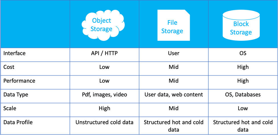
Figure 10.1: Three types of data storage
The first type is object or blob storage. It's vastly scalable, flexible, and REST-based for developing or supporting modern applications. Engineers usually store raw data in this type of storage. The second one is file storage, which is for those applications that require shared file access and a filesystem. The way we interact with file storage is similar to how we interact with the filesystem on our local machine. The last one is block storage. Block or disk storage, unlike the previous two types, cannot be used on its own. It's usually used as a service attached to other applications, such as databases or virtual machines.
Among the three types of data storage, object storage is the most commonly used in modern software and you will most likely be working with object storage when you work in a tech company. In this chapter, we have a lot of opportunities to work with the Amazon Simple Storage Service (S3).
You may be wondering since there are so many cloud providers, why you should choose AWS?
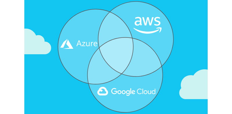
Figure 10.2: Three first-tier public cloud providers
The answer is simple. AWS has a very nice and user-friendly interface for both technical and non-technical people. They also provide free workshops and tutorials about how to leverage their services to build software. AWS is preferable for beginners to learn and use. Knowing how to manage or control services on AWS can help you get on board with the use of other cloud providers faster too.
Now, let's talk about how to access and manage your AWS services. There are mainly two ways to access and control AWS services. The first one is to use the AWS console to interact with its services. The second one, which is also the focus of this chapter, is to programmatically interact with AWS services via the AWS CLI or SDK. As per the following figure, when we log in to the AWS console, we can directly create or terminate services by mouse-clicking and typing in information. However, this approach requires lots of human interaction, which is not a good interface for developing applications. The second approach is for software development purposes. To programmatically access AWS services, you will need to create a role with AWS Identity and Access Management (IAM) with certain permissions so that you can use AWS CLI or SDK to programmatically control your AWS services:
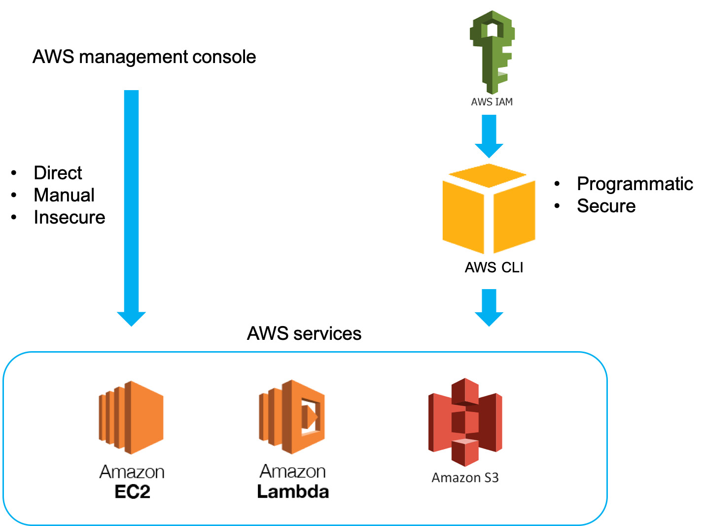
Figure 10.3: Ways to manage your AWS services
Throughout the exercises in this chapter, you will follow the best practices when using cloud services, especially AWS. We will use AWS CLI to interact with AWS services as well as develop workflows using SDK.
In the preceding figure, there are three AWS services. However, we will only be focusing on Amazon S3, which is the object storage service in AWS. To upload your data (photos, videos, documents, and so on) to Amazon S3, you must create an S3 bucket in the AWS region of your choice and give it a globally unique name. AWS recommends that customers choose regions geographically close to them to reduce latency and costs. After an S3 bucket has been created, you can upload any number of objects to the bucket.
In the next exercise, we will create an S3 bucket and upload a file to it.
Exercise 10.01: Uploading a File to an AWS S3 Bucket Using AWS CLI
Imagine that you want to build a data pipeline on a cloud service such as AWS. The first thing you should know is how to upload your files from your local development machine to a cloud storage service such as AWS S3.
We will be using a sample dataset from NYC Open Data. This dataset contains the leading causes of death by sex and ethnicity in New York City (NYC) since 2007. The causes of death are derived from NYC death certificates, which are issued for every death that occurs in NYC. The dataset is provided by the Department of Health and Mental Hygiene (DOHMH). It was created on November 20, 2013, and the last update was on December 9, 2019.
The dataset can be found in our GitHub repository at the following location:
You need to download the New_York_City_Leading_Causes_of_Death.csv file from this book's GitHub repository to your local machine.
Before proceeding with this exercise, we need to set up an AWS account and install AWS CLI, as well as all the necessary configurations. Please follow the instructions on the Preface to install it.
Perform the following steps to complete this exercise:
- Create a directory called Chapter10 for all the exercises in this chapter. In the Chapter10 directory, create a Data directory.
- Move the downloaded New_York_City_Leading_Causes_of_Death.csv file to the Data directory.
- Open your Terminal (macOS or Linux) or Command Prompt (Windows), navigate to the Chapter10 directory, and run following command:
ls
You should get the following output:
Data
The ls command will list the directories and files in the current directory, that is, Chapter10. Inside the Data directory, there should be a New_York_City_Leading_Causes_of_Death.csv file.
- Similarly, we can check whether there is data in our S3 by running the following command:
aws s3 ls
If you're using AWS for the first time, then there will be no data in your S3. Therefore, you should see no output from running the preceding command.
Notice that this command is similar to the command in Step 3. The AWS CLI follows the pattern of aws [service name] [action] [object] [flags]. The command always starts with aws and is followed by a specific service. In our case, the service that we are using is s3. Next to the service is the action you want to perform on this service. Here, our action is ls, which means list files. This ls command is similar to the one from Linux bash.
- Create a bucket by running the following command:
aws s3api create-bucket --bucket ${BUCKET_NAME}
Note
${BUCKET_NAME} is a variable in the command, and you should come up with a bucket name for this exercise. In this chapter, let's set BUCKET_NAME=ch10-data. You will see the ch10-data bucket in the examples throughout the exercises in this chapter.
You should get the following output:
{
"Location": "/ch10-data"
}
If you failed to create a bucket, then you will get the following error:

Figure 10.4: S3 bucket creation failure
If you receive an error, it's not because you did something wrong. It's because the bucket name ch10-data is taken. You just need to give your bucket a more creative name.
The reason why we need to create a new S3 bucket is because an S3 bucket is a store object in S3, which is similar to the concept of a file directory in our operating system. It's a way to organize data. Here, we used s3api to create a bucket. The name of the bucket can be anything arbitrary. Here, we called this bucket ch10-data. When we create a bucket, it will be created in the us-east-1 region by default.
- Verify whether the ch10-data bucket has been created by running the following command:
aws s3 ls
You should get the following output:
2020-01-12 16:03:24 ch10-data
This means there is a bucket named ch10-data in your S3 service. Please ignore the timestamp. The timestamp indicates when the command was run.
- Upload the New_York_City_Leading_Causes_of_Death.csv file to our S3 bucket, ch10-data, by running the following command:
# upload local file to s3 bucket
aws s3 cp ./Data/New_York_City_Leading_Causes_of_Death.csv s3://${BUCKET_NAME}/
You should get the following output:
upload:Data/New_York_City_Leading_Causes_of_Death.csv to s3://ch10-data/New_York_City_Leading_Causes_of_Death.csv
We used the aws s3 cp command to upload the New_York_City_Leading_Causes_of_Death.csv file from our local directory, ./Data, to the S3 bucket path, that is, s3://${BUCKET_NAME}/. The cp command is similar to the one from Linux bash. When you upload files, the AWS CLI follows the pattern of aws s3 [local file path] [s3 bucket path].
- Verify whether the file was uploaded successfully or not by running the following commands:
aws s3 ls s3://${BUCKET_NAME}/
You should get the following output:
2020-01-12 16:15:42 91294 New_York_City_Leading_Causes_of_Death.csv
When you want to list files in an S3 bucket, you can use the AWS CLI by following the pattern of aws s3 ls [s3 bucket path]. It will tell you about all the files from that S3 bucket, provided you have the read access privilege to that bucket.
Alternatively, we can use the AWS console to check if the data has been successfully uploaded or not. Let's look into this.
- Sign in to our AWS console, search for s3 in the search bar, and click the service, as shown in the following figure:

Figure 10.5: Finding the S3 service on the AWS Management Console
This will redirect us to the S3 console and present all of our S3 buckets.
- Click on the first bucket, ch-10-data, as shown in the following figure:

Figure 10.6: List of buckets in our S3
After clicking this bucket, the file should be present inside if it was successfully uploaded, as shown in the following figure:
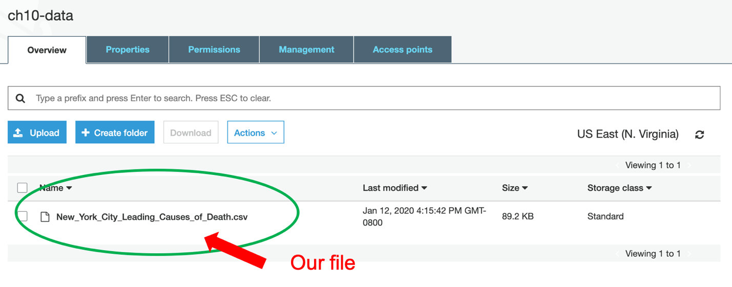
Figure 10.7: List of files in the ch10-data bucket
We can also use the AWS console to interact with our AWS services. The AWS console provides a human-friendly interface and is very easy to understand and use. If you don't know how to perform certain tasks with the AWS CLI command, you can always fall back to using the AWS console and search the documentation for the specific AWS CLI command you want to perform.
Note
To access the source code for this specific section, please refer to https://packt.live/2ZpaKhk.
In this exercise, we learned how to interact with AWS S3 services using the programmatic approach and the AWS console approach. We performed basic tasks on S3 such as creating buckets, listing buckets and files, and uploading files to an S3 bucket.
You will continue to learn about more data tasks in the following exercises. Next, we will learn how to back up our files using S3. We will copy files from one S3 bucket to another.
Exercise 10.02: Copying Data from One Bucket to Another Bucket
Sometimes, we want to back up a piece of data as the source of truth. We can copy the data to another location as a backup so that the original files are free for us to mess with. In this exercise, your task is to create a bucket for backup data and copy the New_York_City_Leading_Causes_of_Death.csv file to the backup bucket.
Perform the following steps to complete this exercise:
- Create a bucket called backup using aws s3api by running the following command:
aws s3api create-bucket --acl private --bucket ${BACKUP_BUCKET}
Note
${BACKUP_BUCKET} is a variable in the command, and you should come up with a bucket name for this backup location in this exercise. In this exercise, let's set BACKUP_BUCKET=storage-for-ai-data-backup. You will see the backup bucket named storage-for-ai-data-backup throughout this exercise.
If the bucket was created successfully, you should get the following output:
{
"Location": "/storage-for-ai-data-backup"
}
If you receive an error again, then it will mostly be because of bucket name collision. This means you just have to give another creative name to this backup bucket.
The preceding AWS CLI command looks different than the one in the previous exercise. We added a new flag, –acl private, to limit the access privilege of this bucket to private, which means any data inside this bucket cannot be read or written by users who don't have access privilege to the S3 bucket. This is not a mandatory requirement; we added it just to keep it private:
Verify if the bucket storage-for-ai-data-backup is created or not by running the following command: aws s3 ls
You should get the following output:
2020-01-12 16:03:24 ch10-data
2020-01-13 20:44:35 storage-for-ai-data-backup
- Create a copy of the file in the backup bucket by running the following command:
aws s3 cp s3://${BUCKET_NAME}/New_York_City_Leading_Causes_of_Death.csv s3://${BACKUP_BUCKET}/
You should get the following output:
copy:s3://ch10-data/New_York_City_Leading_Causes_of_Death.csv to s3://storage-for-ai-data- backup/New_York_City_Leading_Causes_of_Death.csv
We used the aws s3 cp command once more to copy the files from one location to another. In this case, we copied the New_York_City_Leading_Causes_of_Death.csv file from our S3 bucket, s3://${BUCKET_NAME}/, to another S3 bucket, s3://${BACKUP_BUCKET}/. The cp command is similar to the one from Linux bash. When you copy files, the AWS CLI follows the pattern of aws s3 cp [s3 bucket path for source] [s3 bucket path for target].
- Verify whether the file is in the backup bucket or not by running the following command:
aws s3 ls s3://${BACKUP_BUCKET}/
If the file was successfully copied to the backup bucket, you should get the following output:
2020-01-13 21:20:11 91294 New_York_City_Leading_Causes_of_Death.csv
Note
To access the source code for this specific section, please refer to https://packt.live/2ZoZKAI.
In this exercise, we learned how to use the AWS CLI command to perform the copy data task. First, we created a new bucket and then we copied a file from the original S3 bucket to the new S3 bucket.
We will learn how to download files from the S3 bucket using the AWS CLI in the next exercise.
Exercise 10.03: Downloading Data from Your S3 Bucket
Downloading files from an S3 bucket is another very common data task in the day-to-day work of an AI engineer. Whether you are creating a data pipeline or simply performing ad hoc analysis, you will need to download data from cloud storage. In this case, your task is to download data from AWS S3.
Perform the following steps to complete this exercise:
- Open your Terminal (macOS or Linux) or Command Prompt (Windows), navigate to the Chapter10/Data directory, and run the following command:
ls
You should get the following output:
New_York_City_Leading_Causes_of_Death.csv
We downloaded this file in Exercise 10.01, Uploading a File to an AWS S3 Bucket Using AWS CLI. Now, let's remove it and download this file again from our S3 bucket using the AWS CLI.
- Remove the file by running the following command:
rm New_York_City_Leading_Causes_of_Death.csv
- Download the file from our S3 bucket to the Chapter10/Data directory by running the following command:
aws s3 cp s3://${BUCKET_NAME}/New_York_City_Leading_Causes_of_Death.csv ./
Note
${BUCKET_NAME} is a variable in the command, and you should come up with a bucket name for this exercise. In this chapter, let's set BUCKET_NAME=ch10-data. You will see the ch10-data bucket in our examples throughout the exercises in this chapter.
You should get the following output:
download:s3://ch10-data/New_York_City_Leading_Causes_of_Death.csv to ./New_York_City_Leading_Causes_of_Death.csv
You may notice that we used the aws s3 cp command again to download data. This command copies the data from the source location to the destination location. It doesn't matter if the file location is local or remote in S3. To download the data, we essentially copy data from an S3 location to a local file location. Similarly, when we upload data, we are essentially copying data from a local file location to an S3 location.
- Verify the downloaded data by running the ls command in the current working directory:
ls
You should get the following output:
New_York_City_Leading_Causes_of_Death.csv
Note
To access the source code for this specific section, please refer to https://packt.live/2WeswC9.
Now that you've completed the previous three exercises, you can see that the AWS CLI provides a very simple way to control your AWS S3 service and files. However, not everybody is a fan of the bash command. Sometimes, when we develop a data solution, we try to avoid bash because of a lack of testing capability. We want to develop an end-to-end solution in a rather self-contained environment such as developing a data pipeline in Python.
Fortunately, AWS provides many ways for us to access or control its services. Besides AWS CLI, there is an AWS SDK for different programming languages such as Java, Python, Node.js, and so on.
Next, we will be focusing on the Python version of SDK to access and control our S3 services. The Python SDK we are going to use is Boto3, which allows Python developers to write software that makes use of services such as Amazon S3 and Amazon EC2.
In the next exercise, you will be scripting a Python program to upload or download data between your local machine and AWS S3.
Exercise 10.04: Creating a Pipeline Using AWS SDK Boto3 and Uploading the Result to S3
In this exercise, we will develop a data pipeline using a Python script. The script will download the dataset from S3, then find the top 10 leading causes of death and upload the resulting data back to S3.
The source data you will work with is located in the s3://${BUCKET_NAME}/ New_York_City_Leading_Causes_of_Death.csv S3 bucket.
Before proceeding with this exercise, we need to set up the Boto3 AWS Python SDK in the local-dev environment. Please follow the instructions on the Preface to install it.
Perform the following steps to complete this exercise:
- Create a directory called Exercise10.04 in the Chapter10 directory to store the files for this exercise.
- Open your Terminal (macOS or Linux) or Command Prompt (Windows), navigate to the Chapter10 directory, and type in jupyter notebook.
- Create a Python script called run_pipeline.py in the Exercise10.04 directory and add the following code:
import os
import shutil
import boto3
import pandas as pd
if __name__ == "__main__":
# set your bucket name here
# 'ch10-data' is NOT your bucket. It's just an example here
# you should replace your bucket below
BUCKET_NAME = 'ch10-data'
# create s3 resource
s3_resource = boto3.resource('s3')
# downfile from bucket
try:
s3_resource.Bucket(BUCKET_NAME).download_file(
'New_York_City_Leading_Causes_of_Death.csv',
'./tmp/New_York_City_Leading_Causes_of_Death.csv')
except FileNotFoundError:
os.mkdir('tmp/')
s3_resource.Bucket(BUCKET_NAME).download_file(
'New_York_City_Leading_Causes_of_Death.csv',
'./tmp/New_York_City_Leading_Causes_of_Death.csv')
In our run_pipeline.py script, our first step is to download data from an S3 bucket. We used the Python SDK Boto3 to connect with AWS. To access S3 services using Boto3, we created an S3 resource object. Then, we accessed a particular bucket from the resource object with the .Bucket(bucket_name) method. To download data, we use its .download_file(source_file, target_file) method to download the file to our local working directory.
Note
You have probably seen the try-except block elsewhere. It's generally useful when you expect to catch a known exception and handle the exception gracefully. In this case, we expect that the tmp/ directory hasn't been created. So, when an exception is thrown, we create the tmp/ directory first and then perform the download.
- Add the following code snippet to the run_pipeline.py Python script:
# read file with pandas
df = pd.read_csv('./tmp/New_York_City_Leading_Causes_of_Death.csv')
# filter out data with invalid values
df_filterred = df[df['Deaths'].apply(lambda x: str(x).isdigit())]
df_filterred['Deaths'] = df_filterred['Deaths'].apply(lambda x: int(x))
# calculate number of deaths for each year
df_agg = df_filterred.groupby('Leading Cause')[['Deaths']].sum()
# sort and take top 10
df_top10 = df_agg.sort_values('Deaths', ascending=False).head(10)
The next step in this script is to perform calculations. After the file has been downloaded to the tmp/ directory, we use pandas to read the file from the local path. Before we calculate the top 10 death causes, we clean up the data because not all the values in the Deaths column are integers. After we've filtered out the records that aren't integers, we calculate the number of deaths for each cause. We use the pandas .groupby clause to group data into each cause. Then, we apply pandas .sum() to sum up the total number of deaths for each cause. Lastly, we use pandas .sort_values to sort the data based on the number of deaths in descending order and filter to just the top 10 causes using pandas .head(n).
- Add the following code snippet to the run_pipeline.py Python script to upload the result data:
# write new data to new file
df_top10.to_csv('tmp/New_York_City_Top10_Causes.csv')
# upload data to S3
s3_resource.Bucket(BUCKET_NAME).upload_file(
'tmp/New_York_City_Top10_Causes.csv',
'New_York_City_Top10_Causes.csv')
# clean up tmp
shutil.rmtree('./tmp')
print('[ run_pipeline.py ] Done uploading result data to S3 bucket')
The final step of this process is to upload the result data to the same S3 bucket. But we need to write the data to a local file first. To do this, we use the .upload_file (source file, target file) method of Boto3 to upload that file. After that, we delete the tmp folder and print the message for successful uploading.
- Now that you've completed the previous steps, the run_pipeline.py Python script should contain the following code:
run_pipeline.py
13 # create s3 resource
14 s3_resource = boto3.resource('s3')
15
16
17 # downfile from bucket
18 try:
19 s3_resource.Bucket(BUCKET_NAME).download_file(
20 'New_York_City_Leading_Causes_of_Death.csv',
21 './tmp/New_York_City_Leading_Causes_of_Death.csv')
22 except FileNotFoundError:
23 os.mkdir('tmp/')
24 s3_resource.Bucket(BUCKET_NAME).download_file(
25 'New_York_City_Leading_Causes_of_Death.csv',
26 './tmp/New_York_City_Leading_Causes_of_Death.csv')
The complete code for this step is available at https://packt.live/38OYU3e.
At the top of the script, we imported all of the necessary modules. Then, we put all of the code snippets inside the __main__ namespace. The code is executed sequentially under __main__.
- Run the pipeline using the following command:
python run_pipeline.py
You should get the following output:

Figure 10.8: The run_pipeline.py script is successfully running
The script will create a New_York_City_Leading_Causes_of_Death.csv file and upload it to the cloud. You may wonder why there seem to be lots of warnings and complaints. These warnings are from pandas and they suggest their ways of performing certain operations. We could suppress the log from a specific library such as pandas, but this is outside the scope of this book. In our case, we only care about the last line of the output. When we see the last line in the output, it means the script has been executed to the end of the script without any errors occurring.
- Verify whether the data has been successfully uploaded or not by running the following command:
aws s3 ls s3://ch10-data
You should get the following output:
2020-01-12 16:15:42 91294 New_York_City_Leading_Causes_of_Death.csv
2020-01-15 23:22:04 513 New_York_City_Top10_Causes.csv
Note
To access the source code for this specific section, please refer to https://packt.live/38RXftC.
To sum up what we have done so far: we are now able to perform most of the common data tasks such as downloading, uploading, and copying files between our local dev machine and cloud data storage solutions such as S3 using the AWS CLI and the Python SDK, whose library is called boto3.
Cloud data storage solutions are more than just S3 on AWS. AWS also provides other data storage solutions such as relational database services and NoSQL database services. In the next section, we will introduce AWS Relational Database Service (RDS).
Getting Started with Cloud Relational Databases
A relational database is still one of the most used pieces of software in the industry. Many companies use it as a production database to store user information or session logs. Given that Structured Query Language (SQL) is universally well known, many companies also use it as an analytics engine with which business analysts query business metrics to analyze the health of their business or product.
In the AI industry, we also need a relational database to store metadata information for AI modeling experiments. For example, during the model development period, AI engineers often perform model experiments with different training data, different model hyperparameters, and different configurations.
After releasing a production model, AI engineers also want to keep track of what models have been released and their corresponding prediction performance. So, being able to store and organize your AI-related data in a relational database will be tremendously helpful for reproducing research results or performing any retrospective experiment.
However, setting up and operating your databases involves provisioning compute and storage, installing OSes and databases, as well as updating and maintenance. Luckily, AWS RDS makes it extremely easy for us to use a relational database. With this service, we are just a few clicks away from setting up, operating, and scaling our databases:

Figure 10.9: Features of AWS RDS
If you are looking for a solution to store data in a way so that the data is always available, fault-tolerant, and queryable, AWS RDS meets all of these requirements. There are six familiar database engines to choose from regarding AWS RDS, which are Amazon Aurora, PostgreSQL, MySQL, MariaDB, Oracle Database, and SQL Server. Different engines are optimized for different use cases.
In the next exercise, we will create an AWS RDS service via the AWS console. We will use the MySQL engine for this RDS instance.
Exercise 10.05: Creating an AWS RDS Instance via the AWS Console
In this exercise, we will use the AWS console to create an AWS RDS instance, that is, a cloud relational database. Specifically, we will use the RDS MySQL engine. When we create new services in AWS, we usually use the AWS console instead of AWS CLI. This is because creating a new service is a one-time exercise and the AWS console makes creating new services very simple and easy.
This exercise requires an AWS account and the AWS RDS service. This is a free-tier service if your AWS account is less than 12 months old.
Perform the following steps to complete this exercise:
- Log in to the AWS console and search for and click on RDS in the Find Services search bar, as shown in the following figure:

Figure 10.10: Finding RDS on the AWS console
- In the Amazon RDS console, click the Create database option, as shown in the following figure:

Figure 10.11: Creating a database in the RDS console
- On the Create database page, select the Standard Create option, followed by the MySQL option, as shown in the following figure:
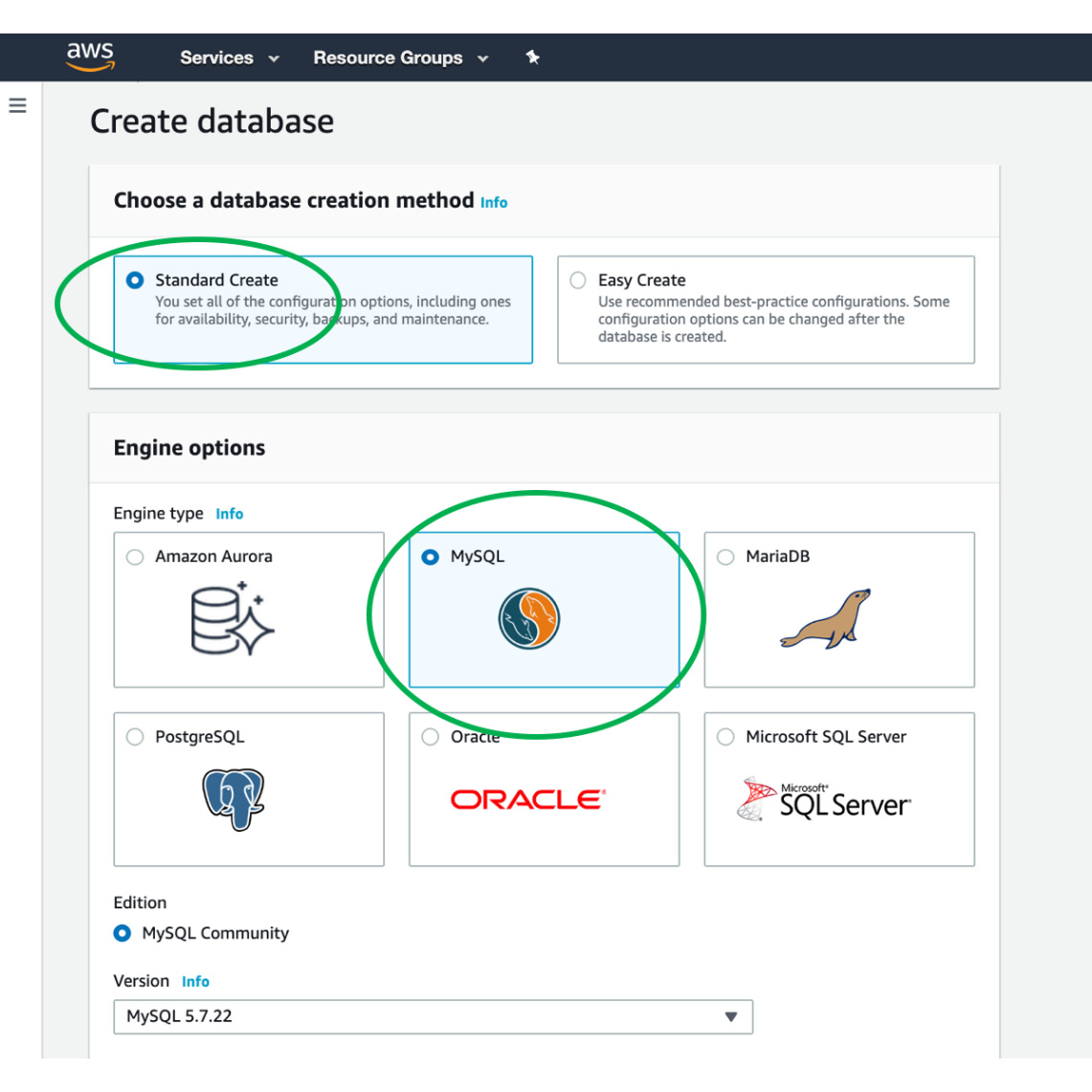
Figure 10.12: Creating a MySQL engine
- In the Templates section, choose Free tier so that you won't be charged:

Figure 10.13: Choosing the Free tier
- In the Settings section, set the values for DB instance identifier and Master username to my-first-rds and my_db_admin, respectively. Also, clear the Auto generate a password checkbox and add a password, as shown in the following screenshot:

Figure 10.14: Configuring settings
Note
Please remember the username and password used in Credentials Settings. We will be using these credentials to access the database later.
- Since we are using Free tier, we can leave the DB instance size, Storage, and Availability & durability sections with their default values, as shown in the following figures:

Figure 10.15: Choosing the instance size

Figure 10.16: Configuring storage

Figure 10.17: Configuring Availability and durability
- In the Connectivity section, expand Additional connectivity configuration and change the Publicly accessible setting to Yes. For the Availability zone, we can choose anyone, as shown in the following figure:

Figure 10.18: Configuring connectivity
By choosing Yes for Publicly accessible, AWS will assign this instance a public IP address, which will allow your local machine to connect to the database. Availability zone refers to the different data centers within a region. In this case, we can choose any.
- Expand the Additional configuration section and enter chapter10 for Initial database name. Keep the default settings for the other options as they are:

Figure 10.19: Additional configuration
- Leave the other sections with their default values and go to the bottom of the console to choose Create database, as shown in the following figure:

Figure 10.20: Create database
- Wait for the Status of your new database instance to show as Available. Then, click the database instance name to show its details:

Figure 10.21: Waiting for the database to be created
When it's finished, you will see the following status:

Figure 10.22: Database created
- In the Connectivity & security section, view the Endpoint and Port of the database instance:

Figure 10.23: Endpoint for RDS connection
Note
Remember to delete this RDS service after finishing the exercises in this chapter, as shown in Step 12. Otherwise, you will be charged if the instance is running for more than 750 hours per month.
- (Do this step after you've finished this chapter.) To delete this service, click the Actions drop-down and select Delete, as shown in the following figure:

Figure 10.24: Deleting the RDS instance
Now that we have Amazon RDS set up, we can create different types of services with our databases. Traditionally, web developers pair up database services with web services to create websites.
In the industry of AI, engineers usually use relational databases to bookkeep different models' performance and experiment results. Recall from Chapter 9, Workflow Management for AI, that we deployed Airflow in our local machine, which is only good for the dev use case. If we want to use Airflow to manage production-level data pipelines, we need to deploy Airflow in the production environment. Instead of using SQLite as our Airflow database, we can use our Amazon RDS as its backend database to manage the metadata for different data pipelines.
But we are not going to deploy Airflow on AWS by ourselves. This type of service deployment or migration usually requires a team of infrastructure engineers. What's more important in this chapter is to be familiar with the AWS CLI so that you can control and manage AWS services.
The way in which programs are connecting to AWS services is through endpoints. To connect to an AWS service, we use an endpoint. An endpoint is the URL of the entry point for an AWS web service. Endpoints are usually made up of IP addresses and ports. With endpoints and user login information, we can essentially log in to the RDS instance and talk to the relational database inside.
In the next exercise, you will be using the AWS CLI to manage your Amazon RDS service and access the RDS database via the MySQL client.
Exercise 10.06: Accessing and Managing the AWS RDS Instance
One of the common tasks when using cloud services is accessing the service itself. In this exercise, we are going to create the service so that we can access it as well as control it. First, we will use the AWS CLI to talk to the service. Then, we will use the MySQL client to connect to our Amazon RDS instance.
Before proceeding with this exercise, we need to set up a MySQL client. Please follow the instructions on the Preface to install it.
Perform the following steps to complete this exercise:
- Check the Amazon RDS service and find its endpoint for the MySQL client using the AWS CLI, as shown in the following code:
# check our RDS instances
aws rds describe-db-instances
You should get the following output:

Figure 10.25: Describing the RDS instance
The preceding output provides all of the information about your RDS services. Here, we only have a single RDS instance, which is named "my-first-rds". The important pieces of information in this giant JSON blob are "MasterUsername", "Endpoint", and its "Address" and "Port". We will need these values to log in to our MySQL instance from our local machine.
- Next, connect our MySQL instance from the local machine using the MySQL client by using the following syntax:
mysql --host ${Endpoint.Address} --port ${Endpoint.Port} -u ${MasterUsername} -p
Note
You have to replace ${variable} with your values in the preceding command. For example, according to the author's credentials, the following command will be used:
mysql --host my-first-rds.c0prwnnsa9ab.us-east- 1.rds.amazonaws.com --port 3306 -u my_db_admin -p
It will ask for a password, as shown in the following output:
Enter password:
You will need to type in the password you created when you created the RDS MySQL instance in Step 5 of Exercise 10.05, Creating an AWS RDS Instance via the AWS Console.
After logging into the MySQL instance, you will observe the following output:

Figure 10.26: Successfully logging in to our RDS instance
Note
If you are unable to log in to your MySQL instance due to the AWS firewall, then you will need to go to the Amazon RDS console to modify the Security group rules, as shown in Step 3 to Step 6.
- (Optional) Log in to the AWS console, navigate to the RDS console, and select your instance, as shown in the following figure:

Figure 10.27: RDS console
- For your instance, you will go to the Connectivity & security section and click on the default (sg-5ce51a16 ) group:

Figure 10.28: Connectivity settings
You will be brought to the Security Group console.
In the Security Group console, click the Inbound tab and then Edit to add a new rule, as shown in the following figure:
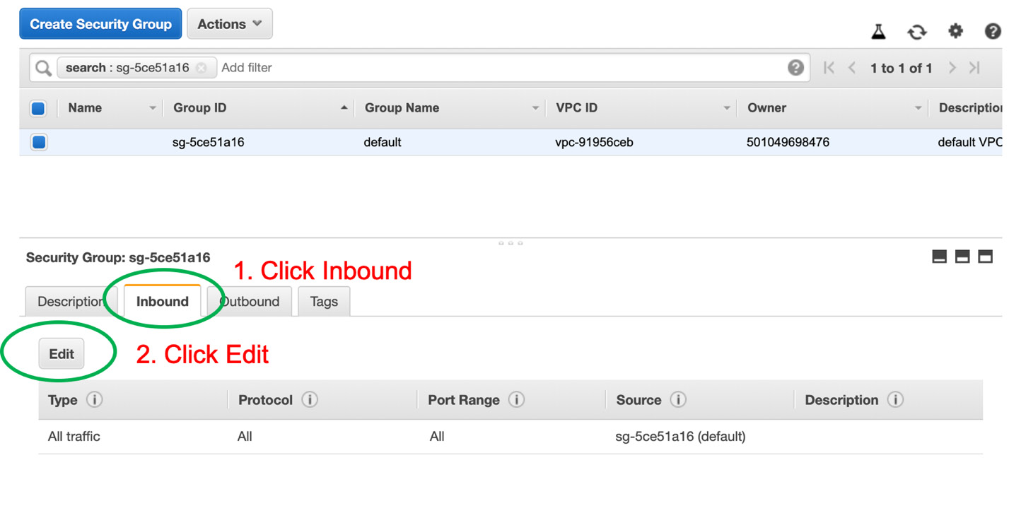
Figure 10.29: Editing the inbound rule for the security group
Now, we can add a new rule for inbound traffic so that the local machine has access to the Amazon RDS instance.
- Click the Add Rule button, select My IP from the Source drop-down, and click Save, as shown in the following figure:

Figure 10.30: Only allowing My IP to be inbound
After you've saved the new rule, you should be able to connect to your MySQL instance from your local machine. Perform Step 2 again to connect to your MySQL instance.
We assume that you are now able to log in to your MySQL instance.
- Query your databases using the following command:
show databases;
You should get the following output:

Figure 10.31: Databases in our RDS instance
If we created our instance correctly in Exercise 10.05, Creating an AWS RDS Instance via the AWS Console, we should be able to see chapter10 as one of the databases.
Note
You might have deleted this instance after finishing Exercise 10.05, Creating an AWS RDS Instance via the AWS Console. If so, you will need to revisit that exercise and recreate the RDS instance for this exercise.
- Select the chapter10 database using the following command:
use chapter10;
You should get the following output:
Database changed
- List the tables inside the chapter10 database by using the following command:
show tables;
You should get the following output:
Empty set (0.09 sec)
However, we will get an Empty set (0.09 sec) this time because we haven't created any tables in this database. But if we import data into this database, we can query information locally via the MySQL client.
- Exit the MySQL client using the following command:
mysql> exit
You should get the following output:
Bye
To avoid any charges, we will delete our Amazon RDS instance.
- Navigate to the RDS console within the AWS console, click Databases on the left-hand pane, and then click the my-first-rds instance, as shown in the following figure:
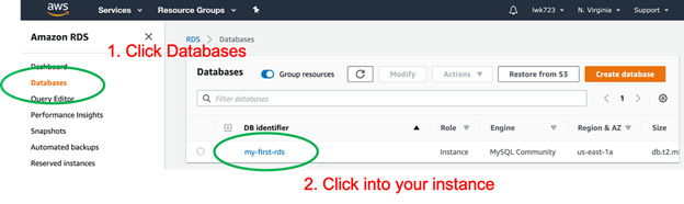
Figure 10.32: RDS console
- In the my-first-rds instance window, click the Actions dropdown and select Delete to remove our RDS service, as shown in the following figure:
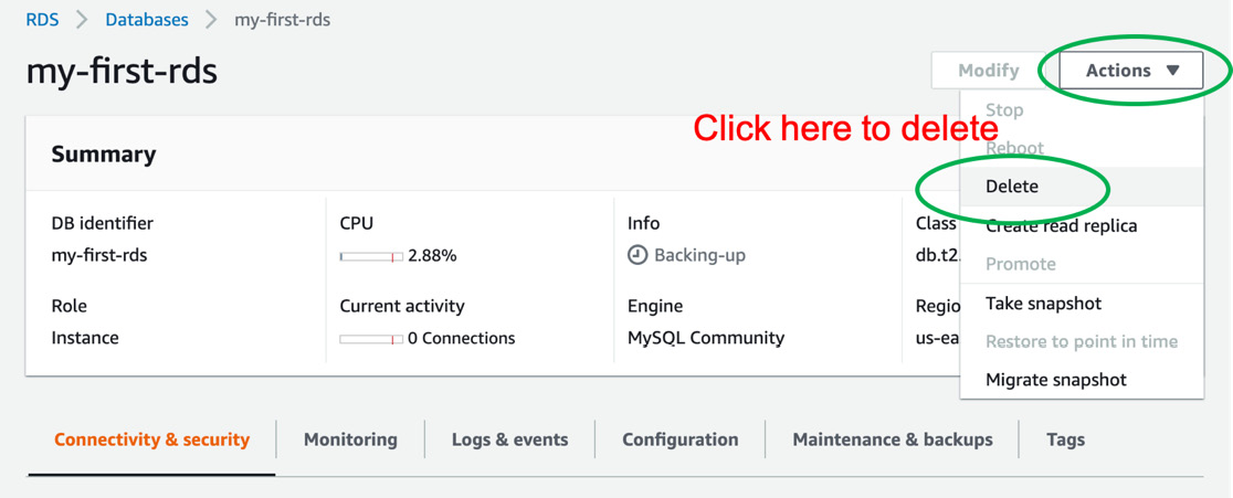
Figure 10.33: Deleting our RDS instance
- In the confirmation popup, select and clear the respective checkboxes and click Delete, as shown in the following figure:
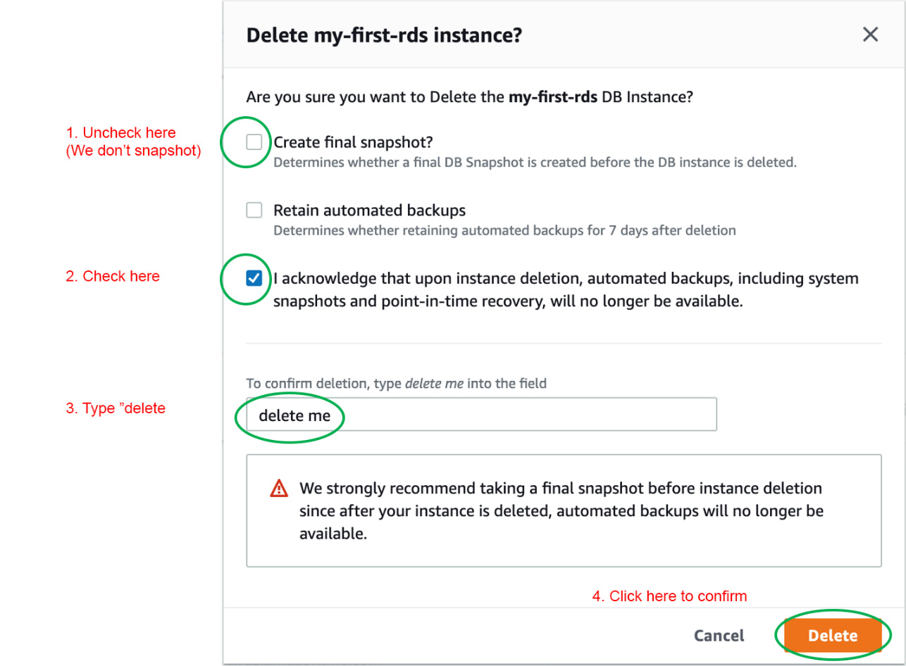
Figure 10.34: Confirmation of the Delete action
Note
To access the source code for this specific section, please refer to https://packt.live/3evEbmo.
Note
In the real world, you will want to create a final snapshot for future recovery. But we don't have any data in this instance, so we don't need to create a snapshot. For more information about database snapshots and how they work, please revisit https://aws.amazon.com/rds/details/backup/.
By completing this exercise, you have successfully implemented the mechanism to access and control the AWS RDS service. First, we used the AWS CLI to get endpoint information. Then, we used the MySQL client to connect with the AWS RDS service to perform database administrative tasks.
Next, we will move on to another type of database, that is, NoSQL databases.
Introduction to NoSQL Data Stores on the Cloud
You may wonder why NoSQL exists when a relational database is powerful enough to store data. As the internet grows, data grows exponentially. And data comes in different shapes and forms. For example, there is more and more long-form document data that needs to be stored somewhere. Not only do we need a database solution to store long-form document data, but it also allows us to query the text data efficiently. Relational databases aren't built for such a use case. Therefore, there are more and more new database technologies emerging, especially in the world of NoSQL databases.
NoSQL databases, also known as non-relational databases, is the other type of database that we can use, as opposed to the relational database. Unlike a relational database, which has a tabular structure and a well-defined entity relationship, NoSQL databases don't require a strict structure or schema. When you are working with a NoSQL database, you generally don't need to think of data in a tabular format with a strict structure. Rather, you will think of data in a loose structure, such as an object in an object-oriented programming language where you can define data in any shape or form you want.
Because of its unstructured nature, NoSQL databases are much more scalable horizontally than traditional relational databases. Therefore, NoSQL databases are especially useful for working with large sets of distributed data:

Figure 10.35: Comparison between NoSQL and relational databases
The preceding figure illustrates the difference between NoSQL and relational databases. Relational databases (on the left) work with tabular data with an explicit schema, while NoSQL databases (on the right) work with document data with an implicit schema. "Implicit" schema usually means the schema is more flexible and allows users to define its schema in an ad hoc fashion.
In the world of NoSQL databases, we can summarize different types of NoSQL database into the following four kinds:
- Key-value data store
- Document data store
- Columnar data store
- Graph data store
Different kinds of data stores accommodate different business use cases and data types. They also differ in terms of read or write performance. Let's understand them better in detail.
Key-Value Data Stores
Key-value data stores are based on the hash map data structure. They implement a data model that pairs a unique key with an associated value. It's extremely simple and performant. Many web applications use a key-value store as their caching system. For example, if engineers want to improve the response time of their website, then they can deploy a caching system alongside the web application to cache user session data or any data that takes time to load.
Some examples of key-value data stores are Redis and Memcached:

Figure 10.36: Key-value data stores
In the cloud era, we don't have to stand up our servers to serve Redis or Memcached services. We simply leverage what the cloud providers are offering. For example, AWS offers ElastiCache, which is a fully managed in-memory data store and cache service. You can choose either Redis or Memcached as its in-memory caching engine. Meanwhile, Google Cloud offers Cloud Memorystore, which is equivalent to AWS ElastiCache.
Document Data Stores
The document data store is frequently used when an application needs to store data in a document format. It usually stores data in a nested format. It doesn't require a schema when developers create or update data.
Due to document data growing on the internet and the use of JavaScript Object Notation (JSON) becoming prevalent in web development, document data stores have become more and more popular.
Let's take a look at some document examples:

Figure 10.37: JSON document format
Here, we have two document records. You can see that they have different schemas. Both of them can be written into the document store.
Today, some of the most well-known document stores are MongoDB, Riak, and ApacheCouchDB. Cloud providers also provide managed services, such as AWS DocumentDB, Google Cloud Datastore, and Azure Cosmos DB.
Columnar Data Store
The columnar data store usually refers to databases that store data by column rather than by row. Traditional databases store data by row because it's easy and intuitive to write data row by row. However, it's less efficient in reading data row by row. When we perform analytical data processing, we usually only select a few columns that are relevant to our analysis. In a row-oriented database, the query engine has to visit every row to fetch the data. However, in the columnar database, the query engine only needs to visit the relevant columns to fetch the data. Therefore, the columnar data store is more efficient in reading data than row-oriented data.
Some well-known examples include Google BigTable, Cassandra, and HBase. Cloud providers offer this type of data store as well. Amazon offers DynamoDB for NoSQL and Redshift for relational.
Graph Data Store
The graph data store is another alternative NoSQL database. The graph is composed of nodes and edges. Nodes represent records, while edges represent the relationship between the records:

Figure 10.38: Nodes and edges in a graph
In a social network setting, records are usernames and edges indicate whether a user is a follower of another user.
Social networks are a good use case for graph stores. Well-known graph data stores include AllegroGraph, IBM Graph, Neo4j, and Titan. For cloud managed services, Amazon offers Neptune and Google Cloud offers Neo4j.
In short, while relational databases store data in a tabular schema, NoSQL databases are built to store data in document format. We will discuss working with data in the document format in the next section.
Data in Document Format
For relational databases, data is usually in a tabular form. The file format for tabular data is usually CSV or TSV. However, data in modern web applications is rarely in a tabular form. For example, when we send a tweet on Twitter, we are effectively making a post request to the tweeter's server with the data being a document format. The data in our post request looks as follows:

Figure 10.39: Data in document format
If you are familiar with web programming, you'll notice that this data is in a JSON format. Data in JSON format naturally manifests the structure of the object in object-oriented programming languages such as JavaScript, Python, and Java. Nowadays, the most common data format that web servers are using between their communications is JSON. For web developers, data in JSON format is preferred to work with than data in tabular format, which means NoSQL databases are also preferable over relational databases.
Most NoSQL databases consume data in JSON format. Due to this, we will need to learn how to create a JSON file in the first place. In the next activity, we will create a simple Python job that performs an analysis and returns data in JSON format.
Activity 10.01: Transforming a Table Schema into Document Format and Uploading It to Cloud Storage
In this activity, we will create a Python job that extracts data from S3, transform the data from table-schema to JSON format, and finally upload the data to S3. Let's imagine that we want to find out the top three death causes for different Race Ethnicity.
Let's use the New_York_City_Leading_Causes_of_Death.csv file to find out the top three death causes for each Race Ethnicity. The data is in tabular format with eight columns, as shown in the following figure:

Figure 10.40: View of the New_York_City_Leading_Causes_of_Death.csv file
We are only interested in the ['Leading Cause', 'Race Ethnicity', 'Deaths'] columns. We will use certain values from these columns to find out the top three death causes for each Race Ethnicity. In this activity, we will use Jupyter Notebook to explore data and use pandas to get the answer. Finally, we will write the result in JSON format. Your final output file should look as follows:

Figure 10.41: Final output data format
Note
The code and the resulting output for this activity has been loaded into a Jupyter Notebook that can be found here: https://packt.live/38TFoCt.
Perform the following steps to complete this activity:
- Use the boto3 AWS SDK to download the source data from the ${BUCKET_NAME} you created in Exercise 10.01, Uploading a File to an AWS S3 Bucket Using the AWS CLI.
- Use the pandas library to read the file, perform data exploratory analysis, and examine the quality of the data. This may require some simple data cleaning.
- Use pandas, groupby, and aggregation, which we learned about in Chapter 9, Workflow Management for AI, to perform the calculation to find out the top three death causes for each Race Ethnicity. Remember to use a Python dictionary to store the result.
- Use json.dump() to serialize the Python dictionary object as you write the data to a JSON file.
- Use the boto3 AWS SDK again to upload the output JSON file to the same S3 bucket.
- Put all of the code snippets together in a single Python script and run it again.
- Use the AWS CLI to verify if the output JSON file has been created. You should get the following output:

Figure 10.42: Final output data has been successfully uploaded to the S3 bucket
Note
The solution to this activity can be found on page 644.
Summary
This chapter introduced some of the most well-known cloud storage solutions, specifically AWS S3. It also covered cloud database solutions for both traditional relational databases and NoSQL databases. Some of the common cloud database solutions are AWS RDS, ElastiCache, DocumentDB, GCP Memorystore, Data Store, and BigTable.
We started by using the AWS CLI in a Terminal to perform common data tasks such as creating a bucket, uploading files, and moving files. Later, we move on to the Python environment, where we used the AWS Python SDK to control AWS resources. At the end of this chapter, we leveraged the practical skills we learned in this chapter and composed an end-to-end pipeline that extracts data from S3, transforms data, and uploads data back to S3. The practical concepts you learned about during these exercises will allow you to build data applications or systems.
In the next chapter, you will continue to build on what you learned in the previous chapters. You will learn how to build AI models that can be combined with data storage systems.
Note
Please remember to delete the RDS service we created in Exercise 10.05, Creating an AWS RDS Instance via the AWS Console and Exercise 10.06, Accessing and Managing the AWS RDS Instance. Otherwise, you will be billed automatically on your credit card after 750 hours.