11. Building an Artificial Intelligence Algorithm

Overview

We will start this chapter by introducing the most basic form of machine learning model: the linear regression model. We will use batch gradient descent in NumPy to train a regression model. Then we will get started with the popular deep learning framework PyTorch. Toward the end of the chapter, we will delve into one of the most exciting fields in deep learning research: reinforcement learning, specifically the deep Q-learning algorithm. Lastly, we will learn how to build a deep Q-learning algorithm to solve classic reinforcement learning problems, and we will learn how to improve the algorithm by implementing a double deep Q-learning algorithm in an activity.

By the end of this chapter, you will have a comprehensive understanding of how an Artificial Intelligence (AI) algorithm is built and trained with different implementations such as NumPy and PyTorch. Both NumPy and PyTorch are Python-based scientific computing packages. AI practitioners use them very frequently in the field of deep learning research. You will learn about the nuts and bolts of AI algorithms along with the best practices in training an AI model.

Introduction

In previous chapters, we learned about various hardware and software infrastructures for AI practices. We learned about different databases and data solutions as well as their use cases. We learned about big data computing engines such as Spark, which allows engineers to process web-scale data. We also learned about using workflow management systems such as Airflow to manage data pipelines at scale. We also learned a lot about cloud data solutions and how to leverage cloud data storage and perform basic data-related tasks.

This chapter will focus on the science and the mathematical side of artificial intelligence. Without a proper understanding of the theory that underpins AI, we simply cannot build a robust AI application. If we can understand the math and science behind AI, then we will be able to apply different algorithms to solve different real-world problems. With the skills you will gain from this chapter, you will be able to innovate new AI algorithms to solve new problems.

Machine Learning Algorithms

There are four main types of learning algorithms:

• Supervised learning algorithm: This is trained to predict an outcome for a given set of input features. It's well studied and widely used in many areas such as spam classification, fraud detection, and product recommendation.
• Unsupervised learning algorithm: This analyzes the underlying patterns or structure of data and groups data into clusters. Examples are outlier detection, fraud detection, and dimensionality reduction.
• Semi-supervised learning: This falls between supervised learning and unsupervised learning. It's intended to boost learning accuracy for a supervised learning model by mixing unlabeled data.
• Reinforcement learning algorithm: This is trained to play a "game." It learns to take a "smarter" action at each step in a game so that it will eventually win the game. Examples are AlphaGo, robot control, and quantitative trading.

This chapter will focus on supervised learning and reinforcement learning. We will start by learning the fundamental theory and basic techniques in training a supervised learning model. Then we will get hands-on experience in building a reinforcement learning algorithm to play a classic control game in OpenAI Gym.

Model Training

There are many different machine learning models for each of those four types of learning algorithms. Machine learning models rely on some forms of mathematical/statistical models. When we train models, it means we use an algorithm to find out the model's unknown parameters. Scientifically speaking, we cannot definitively find out the ground truth for unknown parameters. Instead, we can only estimate the unknown parameters as closely as possible to the ground truth by using mathematical/statistical methods on sample data. Estimating unknown model parameters is equivalent to solving a mathematical equation whose solution comes in one of two forms: closed or non-closed.

Closed-Form Solution

Some algorithms' mathematical models have closed-form solutions. A model with a closed-form solution can be solved by expressing the model parameters analytically in terms of a finite number of certain "well-known" functions. A classic example is a linear regression model. Training a linear regression model is equivalent to solving a quadratic matrix equation in linear algebra. The quadratic matrix equation is derived from a method called Ordinary Least Squares (OLS). The OLS method essentially tries to minimize the distance between model predictions and ground truth values. Through a series of linear algebra transformations, the minimization solves a quadratic equation, which always has a closed-form solution. To further simplify the problem, let's consider a simple linear regression model, shown in the following figure:

Figure 11.1: Linear regression solved by OLS

In the preceding figure, the left cell is the mathematical form of a simple linear regression that has only two parameters, α, and β. Parameter α is known as the bias and parameter β is known as the weight of input x. The term Ɛ indicates errors that exist in a model. The right cell shows the closed-form solution for OLS.

Non-Closed-Form Solutions

Note that most other machine learning models do not have closed-form solutions. To train a model with a non-closed-form solution, we need to employ other techniques to estimate model parameters. For example, some of the well-known methods are Newton's method, convex optimization, and stochastic optimization. In the field of machine learning and deep learning, the most common technique is gradient descent from stochastic optimization. If you are not familiar with it, don't worry. In this chapter, we will be spending lots of time on gradient descent. Besides, we will implement gradient descent techniques in our learning algorithms to train models too.

Gradient Descent

Before we dig into what gradient descent is, let's answer the question of why gradient descent is one of the most important techniques in machine learning. For the sake of simplicity, let's use the linear regression model as an example to illustrate. Let's say we are building a model to predict house prices given the area of the house. The mathematical model is as follows: predicted house price = bias + weight*area of the house.

When we initialize the model, we need to initialize the values for the bias and the weight. Usually, we draw random numbers for the initialization of biases and weights. So, now the model becomes the following: predicted house price = 9 + 5*area of the house.

Bias = 9 and weight = 5 are not ideal model parameters to predict the house price. Currently, the model could be extremely wrong about its house price prediction. It is not even close to being accurate. At the same time, there might exist an ideal value for the bias and an ideal value for the weight, such that the model predicts house prices accurately. So, now the question is this: how do we train the model to make it become an accurate model?

Training the model means we need to update the values for the bias and the weight in a way such that the model prediction gets closer and closer to being accurate. So, let's measure how wrong the model is by measuring the distance between a model prediction of a house price and the actual price of a house. The smaller the distance, the more accurate the model is. This means we need to update the values for the bias and the weight in such a way that the distance between the model prediction and the actual house price is minimized. Now the model training procedure turns into a minimization problem in the mathematical model, as shown in the following figure:

Figure 11.2: Gradient descent

The preceding figure nicely illustrates what gradient is and how gradient descent solves the minimization problem. w represents the weights in our house price prediction model, so we can express the distance, J(w), between the prediction and the real house price in terms of w. The model with its initial weight is far from being accurate and has a huge distance from the minimum. The fastest way for the model to achieve the minimum is through a process called gradient descent. The gradient here is the steepest direction along the path to the minimum; gradient descent is also known as steepest descent. According to Figure 11.2, when we train the model, we are updating the values of weights with their gradients iteratively in a way such that J(w) gradually reaches the minimum step by step.

Note that J(w) is usually the loss function to measure the distance between the model prediction and the ground truth. Depending on the model type, there are various loss functions that you can choose from. For example, Mean Squared Error (MSE) is usually the go-to loss function for a regression model, and cross-entropy is used for a classifier model. We will be working with regression models, so we will focus on MSE in this chapter. The formula for MSE is as follows:

Figure 11.3: Definition of MSE

In a simple linear regression model, y=mx+b, where m is the weight and b is the bias, the gradient of the MSE loss function in the linear regression model is represented by two partial derivatives. One is the partial derivative of MSE with respect to the weight and the other is with respect to the bias. The formula is as follows:

Figure 11.4: The gradient of MSE with respect to the weight and bias in linear regression

During gradient descent, we will update the weight and bias by subtracting their corresponding partial derivatives. As we update the weight and bias, the loss will continue to reduce until it converges to a small value, just like the global cost minimum Jmin(w) shown in Figure 11.2.

In short, gradient descent is an optimization algorithm used to minimize the distance by iteratively updating a model's weights to the direction of steepest descent as indicated by the gradient.

Let's now get some hands-on experience with gradient descent. We will implement gradient descent in our first exercise.

Exercise 11.01: Implementing a Gradient Descent Algorithm in NumPy

Imagine you are an AI engineer working on a machine learning research project. The first project is a warm-up project and you will create a model and build a gradient descent algorithm to train the model. You may wonder why we would want to build one from scratch when there are already many open source machine learning libraries that have implemented gradient descent. While being practical is crucial to success in engineering, an understanding of the mathematical theory that underpins AI plays a critical role in the success of an AI engineer. You will have a much higher chance of innovating new AI techniques than your peers if your fundamentals are solid.

When we are building a new algorithm from scratch, we want to build it in such a way that it should work for a very simple/naïve model with minimal assumptions. Building something that works for a base case is always a good start. In this case, our base case is a linear regression model. If we build something that doesn't even work for linear regression, then it probably won't work for more complicated models, such as neural networks and deep learning models. At the end of the exercise, our gradient descent algorithm should be able to train the linear regression model and calculate the model's weights to be as close as possible to the ground truth.

To get started with building a gradient descent algorithm, we will use one of the most popular scientific libraries, NumPy. NumPy is a Python library for scientific computing and manipulating multi-dimensional arrays.

Before proceeding to the exercise, we need to set up a data science development environment. We will be using Anaconda. Please follow instructions in the Preface to install it.

Perform the following steps to complete the exercise:

1. Create a Chapter11 directory for all the exercises in this chapter. After creating the Chapter11 directory, change your working directory from your current working directory to Chapter11.
2. In the Chapter11 directory, launch a Jupyter Notebook in your Terminal (macOS or Linux) or Command Prompt (Windows).
3. After the Jupyter Notebook is launched, let's create a new directory named Exercise11.01.
4. Select the Exercise11.01 directory, then click New -> Python3 to create a new Python 3 notebook.
5. Inside the Python 3 notebook, import all necessary modules as shown in the following code:

   import numpy as np

   import matplotlib.pyplot as plt

   plt.style.use('ggplot')

   We will import the matplotlib module for our first exercise. The matplotlib module is a very handy tool when it comes to data visualization in the realm of data science. We will be using it to visualize the training data, the model, and the training process in the following steps.

   The plt.style.use('ggplot') line configures the plotting style for all of the following plots in the notebook. The ggplot style will render the plots with a gray background with white grid lines. You will see the plot style in later steps.

6. Next, create some synthetic data for training our linear regression model. Use the NumPy.random.uniform method to generate sample data from a uniform distribution and the NumPy.random.normal method to generate artificial noise data from a normal distribution as shown in the following code:

   # set random seed

   np.random.seed(9)

   # draw 100 random numbers from uniform dist [0, 1]

   x = np.random.uniform(0, 1, (100, 1))

   # draw random noise from standard normal

   z = np.random.normal(0, .1, (100, 1))

   # create ground truth for y = 3x - 1

   y = 3 * x - 1 + z

   NumPy supports the drawing of random numbers for various statistical distributions. We used uniform distribution to draw input values for x. Uniform distribution is similar to the probability distribution of rolling a die, where every number from 1 through 6 has an equal likelihood of being drawn. In our case, any real number between 0 and 1 is drawn with equal likelihood. We choose to use the standard normal to generate artificial noise data, z, to mimic Gaussian noise, which is the most common form of noise in a natural dataset.

   Now let's understand the structure of the data. When we are working with an array or matrix, one way to put data into perspective is to examine the array's shape property. This tells you the number of elements for each dimension in an array. For example, an array with shape (2, 3) means its first dimension has two elements and its second dimension has three elements, which means the array is a 2 x 3 two-dimensional array.

   x is an array with shape (100, 1) that we created from a uniform distribution with the parameters (0, 1). z is also an array with the shape (100, 1) from the normal distribution and it represents noise in the sample data. y is also an array with the shape (100, 1) created by the model of 3x -1. Note that y is what our model is trying to predict for a given value of x. The ground truth model parameters are weight = 3 and bias = -1.

   Notice that we also seeded the randomness in the first line with np.random.seed(9) so that you can reproduce the same results when you run the same code. In the following steps, we will be pretending that we don't know the values of the model parameters. We will be training our linear regression model to find out the best estimates of the weight and bias.

7. Let's split the syntactic data into two sets as shown in the following code:

   # split data into train and test

   x_train, y_train = x[:80], y[:80]

   x_val, y_val = x[80:], y[80:]

   One set is for model training and the other set is for validating how accurate our model is after training. Let's slice the array to split the data. We are doing an 80/20 split for training and validation, which is the most common model validation strategy. Another model validation strategy is cross-validation. However, it is not included in the scope of this chapter.

8. Let's visualize the training and validation sets using the matplotlib data visualization module as shown in the following code:

   # visualize

   fig, axes = plt.subplots(nrows=1, ncols=2, figsize=(12, 4))

   axes[0].scatter(x_train, y_train, label='train', color='b')

   axes[0].set_title('Train')

   axes[0].set_xlabel('x')

   axes[0].set_ylabel('y')

   axes[0].legend()

   axes[1].scatter(x_val, y_val, label='val', color='g')

   axes[1].set_title('Validation')

   axes[1].set_xlabel('x')

   axes[1].set_ylabel('y')

   axes[1].legend()

   fig.tight_layout()

   You should get the following output:

   

   Figure 11.5: Visualization of training and validation data

   Let's pretend we don't know that the true model is a linear model with weight = 3 and bias = -1 and that we need to create a model to predict the y value for any given x. According to the data visualization, we can make a strong assumption that the data follow a linear model pattern. So, let's create a linear regression model in the next step.

9. Let's initialize a linear regression model by drawing two random numbers for the model's weight and bias, as shown in the following code:

   # create trainable parameters for the model

   weight = np.random.randn(1)

   bias = np.random.randn(1)

   print("model with weight = {} and bias = {}"

         .format(weight, bias))

   You should get the following output:

   model with weight = [-1.03600638] and bias = [-0.13392398]

10. Let's use this initial linear model to predict y values for x values in the training data and visualize this model prediction accuracy as shown in the following code:

    # let's predict y value for the training data using initial model

    y_hats = [bias + weight * x for x in x_train]

    # let's visualize the initial model

    plt.scatter(x_train, y_hats, color='b')

    plt.title('Initial model')

    plt.xlabel('x')

    plt.ylabel('y')

    plt.tight_layout()

    You should get the following output:

    

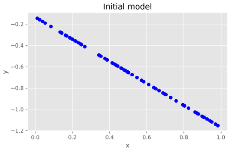
    Figure 11.6: Visualization of the newly initialized linear model

    Notice that the initialized linear model is almost the opposite of the true model (y=3x-1), which is manifested by the training and validation data in Figure 11.5. As the initialization of the model is random so the model is opposite to the true model. We will be training the model with the gradient descent technique and updating the weight and bias accordingly. With gradient descent, we adjust the weight and bias step by step so that the model gets closer and closer to the ground truth. You will see how this model improves and gets closer to the ground truth.

11. Next, we will implement the gradient descent algorithm to update the model. The algorithm is implemented in the following code:

    # set training routine

    lr = 1e-1

    n_epochs = 500

    # keep records

    losses = []

    val_losses = []

    # train model

    for epoch in range(n_epochs):

        print("[ epoch ]", epoch)

        # forward pass

        yhat = bias + weight * x_train

        # calculate the error

        error = (y_train - yhat)

        # calcuate loss function

        loss = (error ** 2).mean()

        losses.append(loss)

        print("[ training ] training loss = {}"

              .format(loss))

        # calcuate the gradients for model's

        #trainable parameters

        bias_grad = -2 * error.mean()

        weight_grad = -2 * (x_train * error).mean()

        # perform gradient descend

        bias = bias - lr * bias_grad

        weight = weight - lr * weight_grad

        # calculate validation loss

        yhat = bias + weight * x_val

        error = (y_val - yhat)

        val_loss = (error ** 2).mean()

        val_losses.append(val_loss)

        print("[ eval ] validation loss = {}".format(val_loss))

    print("linear.weight = {}, linear.bias = {}"

          .format(weight, bias))

    You should get the following output:

    

    Figure 11.7: Logs of the model training process

    Note

    We will have loads of output data with 500 iteration results. We have only taken the last section of it in the preceding figure.

    The output is logging training loss and validation loss for each training epoch so that we can see how the model is improving and the loss is reducing over time. The final weight is 2.98244477 and the bias is -0.97201471, which are very close to the ground truth of our model, y = 3x - 1.

    In the gradient descent algorithm, we create a for loop for 500 iterations. This means the weight and bias are being updated 500 times. In deep learning terminology, one iteration of the parameter update with the entire input dataset is also known as one "epoch." In each epoch, we predict y values as yhat for x values for all training data. Then we calculate the error and loss functions between the ground truth and the model's predictions. We then calculate the loss function's gradient, which is a partial derivative for the weight and bias. We update the weight and bias by subtracting the learning rate * gradient. For each epoch, the gradient always points us downhill and the loss is continuously reduced until it converges on a very small number. After 494 epochs, as shown in Figure 11.7, the training loss is reduced and converges on a very small number, 0.0086. When we see that the loss is converged to a small number, it means the model training is finished.

    Notice we did not update the weight and bias by subtracting their gradients directly. Instead, we subtract a much smaller amount of the gradient, which is the learning rate * gradient; the learning rate is always less than one. The learning rate is a very important hyperparameter of gradient descent. It represents a learning step, and the larger the learning rate, the quicker the loss is minimized. However, the loss may not be able to converge if the learning rate is too large. We set the learning rate to be 0.1 here so that the loss is minimized smoothly.

12. Let's visualize how the MSE loss function is minimized during gradient descent as shown in the following code:

    # visualize the loss during gradient descent

    plt.scatter(range(n_epochs), losses, label='train_loss', color='b')

    plt.scatter(range(n_epochs), val_losses, label='val_loss', color='r')

    plt.legend()

    plt.title('Loss')

    plt.xlabel('epochs')

    plt.ylabel('mse')

    plt.tight_layout()

    You should get the following output:

    

    Figure 11.8: Minimizing the loss function using gradient descent

    We can see that both the training loss and validation loss drop very quickly from the first epoch to the 100th epoch. After the 100th epoch, the loss starts to converge to a small number and becomes more and more stable. The goal of a training model with a gradient descent technique is to minimize the loss until the point where the loss starts to converge and flatten out. In this case, the model reaches a minimum around the 130th epoch. This means we effectively only need 130 epochs to train this linear regression model.

13. Finally, let's compare the trained model prediction against the ground truth in the validation data by running the following code:

    # let's predict y value for the validation data using the trained model

    y_hats = [bias + weight * x for x in x_val]

    # let's visualize the intial model

    plt.scatter(x_val, y_hats, label='prediction',

                color='b')

    plt.scatter(x_val, y_val, label='ground truth',

                color='r')

    plt.legend()

    plt.title('Trained model')

    plt.xlabel('x')

    plt.ylabel('y')

    plt.tight_layout()

    You should get the following output:

    

Figure 11.9: Final model prediction versus ground truth

We can see that the model is predicting very closely to the ground truth. The reason why the model isn't able to predict with perfect accuracy is that there is artificial noise in the training data, which was created on purpose. In the real world, there is always noise in the data. The best we can do is to estimate the model weight and bias as closely as possible to the ground truth by minimizing the loss function. That's why gradient descent is such a powerful technique in model training.

Note

To access the source code for this specific section, please refer to https://packt.live/38SejQp.

In this exercise, we first created a syntactic dataset and linear regression model using NumPy. Then we implemented a gradient descent algorithm to successfully train the linear regression. At the end, we compared our trained model with the ground truth by using the Matplotlib library to create two scatter plots for comparison.

You need to figure out the gradient function based on the model. We are using the simplest model, linear regression, in this exercise, and it's fairly easy and straightforward to derive gradient by hand in this case. We can analytically calculate the gradient in this case because the OLS technique for training a simple linear regression model has a closed-form solution. But if our model were a deep neural network, then calculating its gradients would be an ordeal. There are thousands or even millions of parameters in a typical neural network model. Calculating the partial derivatives for all its parameters would be the next ordeal that we would have to tackle. This is when deep learning libraries such as TensorFlow and PyTorch come to the rescue. With deep learning libraries, AI engineers can do machine learning/deep learning research at scale with ease. They can innovate new models and algorithms at a much faster iteration speed.

Next, you will be introduced to PyTorch, and we will take you through how PyTorch can help you build an AI algorithm.

Getting Started with PyTorch

PyTorch is one of the most popular open-source deep learning libraries in the world right now. It's known for its fast iteration, model ideation, and prototyping. As a result, many AI researchers or engineers implement their state-of-the-art deep learning models through the PyTorch library or its ecosystem. PyTorch has a large machine learning community and its community continues to grow and mature. Another popular deep learning framework is TensorFlow. TensorFlow gained its popularity a little earlier than PyTorch. Let's compare the differences in their core features:

Figure 11.10: PyTorch versus TensorFlow

Generally speaking, PyTorch is more development-friendly and TensorFlow is more deployment-friendly. Both are very powerful deep learning frameworks. If you want a better development and research experience, PyTorch is a better fit for you. On the other hand, if you want to deploy your models to production, then TensorFlow is a more mature option. That being said, you can use TensorFlow to achieve everything you can do in PyTorch, but with more effort.

From the user experience perspective, PyTorch is a very intuitive library for building mathematical models, especially for people with a math background. This is one of the reasons why we chose PyTorch for the exercises in this chapter. Using PyTorch helps us to build up the mathematical intuition for building and implementing mathematical algorithms and deep learning models.

Note

For more information about PyTorch, please visit https://pytorch.org/.

PyTorch, similar to NumPy, is a Python library for scientific computing. While NumPy serves as a generic scientific computing tool, PyTorch is built for deep learning modeling and neural networks. NumPy makes multi-dimensional array computation extremely efficient on CPUs and PyTorch allows tensors and their computation to run on GPUs. Deep learning models usually consist of tens of layers of tensors, which results in thousands of parameters in a single model. Running computation for thousands of parameters can be very slow sometimes. However, running such computations on a GPU is way more efficient because a GPU has hundreds of small cores to achieve higher parallelization, while a CPU usually has four to eight cores to parallelize.

You may not be familiar with the term "tensor." A tensor is a mapping between two algebraic objects in a vector space. An algebraic object can be a scalar, a vector, or a multi-dimensional array. A neural network model such as an image classifier is made of tensors. A model maps an image's pixels to labels of the objects inside the image. For example, if you feed the pixel data of an image of a car to an image classifier model, then the model will tell you there is a car in the image.

In terms of mathematical representation, a tensor is also an algebraic object in a vector space. Let's revisit our baseline linear regression model to illustrate:

Figure 11.11: Linear regression model

In the mathematical expression, α is the bias, and β is the weight in the linear regression model. In Exercise 11.01, Implementing a Gradient Descent Algorithm in NumPy, α is a scalar in NumPy and so is β. Now, in the world of PyTorch, α and β are tensors. So is every algebraic object in PyTorch.

Now let's get into the meat of topic about why PyTorch as a deep learning library, compared to NumPy, is more useful for training deep learning models. It's because PyTorch has the autograd package. autograd is used for automatic differentiation. Recall in Exercise 11.01, Implementing a Gradient Descent Algorithm in NumPy, that when we perform gradient descent, we need to calculate the partial derivatives for both the weight and the bias, meaning we need to differentiate the loss function with respect to the weight and the bias. There is no automatic differentiation in NumPy; so we were calculating the partial derivatives by hand and we hardcoded it in the gradient descent algorithm. With PyTorch, the gradient is automatically calculated by its autograd library.

To understand how automatic differentiation is achieved in PyTorch's autograd package, we need to first understand how a computer interprets a model. A computer interprets a model through a computational graph. Let's use our simple linear regression model, y=mx+b, to illustrate the computational graph, as shown in the following figure:

Figure 11.12: Computational graph for a simple linear regression model

In the preceding figure, starting from the top, are the weight (m), the bias (b), and the input data (x). They are also known as the graph leaf nodes in the computational graph. The circles represent the mathematical operators in the graph. Operators connect leaf nodes and produce the final output as y, which is the head in the graph.

During model training, we will need to find out the gradients by differentiating the loss with respect to the bias (b) and the weight (m). When we use PyTorch to build a model, PyTorch's autograd package will register nodes and operators into a computational graph so that it keeps track of the gradients and automatically calculates them for you.

Now we know why PyTorch is a good tool for machine learning model training. In the next exercise, let's upgrade our gradient descent algorithm from Exercise 11.01, Implementing a Gradient Descent Algorithm in NumPy, and use PyTorch to perform gradient descent instead of NumPy.

Exercise 11.02: Gradient Descent with PyTorch

In this exercise, we will improve our gradient descent algorithm with PyTorch's autograd package. Fortunately, we implemented the entire skeleton of the gradient descent algorithm to train the linear regression model in Exercise 11.01, Implementing a Gradient Descent Algorithm in NumPy. Now we will only change the code in places that require the use of PyTorch to perform automatic differentiation while keeping most of the skeleton unchanged.

To be more specific about what we need to do in this exercise, we will need to do the following:

• Convert the data and the model from a NumPy object to a PyTorch tensor object.
• Replace the hardcoded gradient calculation part with PyTorch's autograd implementation.
• Rerun the model training and verify that the trained model is close to the ground truth.

Before proceeding to the exercise, we need to install the data science environment from Anaconda and the PyTorch package. Please follow the instructions in the Preface to install them.

Perform the following steps to complete the exercise:

1. In the Chapter11 directory, launch a Jupyter Notebook in your Terminal (macOS or Linux) or Command Prompt window (Windows).
2. After the Jupyter Notebook is launched, create a new directory named Exercise11.02. Inside the Exercise11.02 directory, create a Python 3 notebook.
3. Inside the Python 3 notebook, import all necessary modules as shown in the following code:

   import numpy as np

   import torch

   import matplotlib.pyplot as plt

   plt.style.use('ggplot')

   device = 'cuda' if torch.cuda.is_available() else 'cpu'

   We will be using NumPy and Matplotlib again in this exercise. Besides this, we will use the PyTorch library by importing torch into our Jupyter Notebook environment. At the last line, torch.cuda.is_available() returns True if torch detects that there is a GPU device available on your machine; otherwise, it returns False. So, the device variable is a string with a value of either cuda or cpu. You will find out how we will use this variable in later steps in the exercise.

4. Generate some syntactic data for the linear regression model as shown in the following code:

   # set random seed

   np.random.seed(9)

   # draw 100 random numbers from uniform dist [0, 1]

   x = np.random.uniform(0, 1, (100, 1))

   # draw random noise from standard normal

   z = np.random.normal(0, .1, (100, 1))

   # create ground truth for y = 8x - 3

   y = 3 * x - 1 + z

5. Split the data into two sets, train and test, as shown in the following code:

   # split data into train and test

   x_train, y_train = x[:80], y[:80]

   x_val, y_val = x[80:], y[80:]

   print(type(x_train))

   You should get the following output:

   <class 'numpy.ndarray'>

   We use NumPy to create the syntactic data, so the type of data is a numpy.ndarray object. In this exercise, we need to work with PyTorch, so we will move the data to a new object type (tensor) that PyTorch can work with in the next step.

6. Next, we will convert the data from a NumPy object to a PyTorch tensor object as shown in following code:

   # move data from numpy to torch

   x_train_tensor = torch.from_numpy(x_train).float().to(device)

   y_train_tensor = torch.from_numpy(y_train).float().to(device)

   x_val_tensor = torch.from_numpy(x_val).float().to(device)

   y_val_tensor = torch.from_numpy(y_val).float().to(device)

   print(type(x_train_tensor))

   You should get the following output:

   <class 'torch.Tensor'>

   Now both the training data and the validation data are converted to torch.Tensor objects. The torch.from_numpy() function call is a very handy method for converting a NumPy array object to a PyTorch tensor object. .float() means we want the converted data type to be of the float type. .to(device) will move the tensor from its current device to the desired device. For example, if a GPU is available on your machine and you want to move your tensor from the CPU to the GPU, then you will use the .to('cuda') method. This explains why we set the device variable to either cpu or cuda in step 3 at the last line.

7. Now we will initialize our linear regression model parameters, weight, and bias, in PyTorch as shown in the following code:

   # create trainable parameters for the model

   weight = torch.randn(1, requires_grad=True,

                        dtype=torch.float, device=device)

   bias = torch.randn(1, requires_grad=True,

                      dtype=torch.float, device=device)

   print(weight, bias)

   You should get the following output:

   tensor([-1.0688], requires_grad=True) tensor([-0.6226],

   requires_grad=True)

   Notice that we set requires_grad=True when we initialize the tensors for weight and bias. In PyTorch, tensors with the requires_grad=True attribute will be registered into the PyTorch computational graph where any graph leaf tensor is automatically differentiable. This will allow us to automatically compute the gradients for the weight and the bias, which will make gradient descent much easier.

8. After the data and the model are created, we now can train the linear regression model by performing gradient descent. The following code implements the gradient descent algorithm:

   ex2-notebook.ipynb

   # set training routine

   lr = 1e-1

   n_epochs = 500

   # train model

   losses = []

   val_losses = []

   for epoch in range(n_epochs):

       print("[ epoch ]", epoch)

       yhat = bias + weight * x_train_tensor

       error = y_train_tensor - yhat

       loss = (error ** 2).mean()

       losses.append(loss.item())

       print("[ training ] training loss = {}".format(loss))

       # calculate gradients

       loss.backward()

       # update weight and bias

       with torch.no_grad():

           bias -= lr * bias.grad

           weight -= lr * weight.grad

       # zero out grads

       bias.grad.zero_()

       weight.grad.zero_()

   The full code is available at https://packt.live/30bU0t2.

   You should get the following output:

   

   Figure 11.13: Logs of the model training process

   Note

   We will have loads of output data with 500 iteration results. We have only shown the last section of it in the preceding figure.

   The log output is similar to the one in Exercise 11.01, Implementing a Gradient Descent Algorithm in NumPy, where both training loss and validation loss are minimized over time. The final weight is 2.9827 and the bias is -0.9722, which are again very close to the ground truth of our model, y = 3x – 1.

   If we compared the code snippet to step 11 in Exercise 11.01, Implementing a Gradient Descent Algorithm in NumPy, you will notice that the skeleton of the training routine is almost the same and the only difference is the part that updates the gradients, as shown in the following code:

       # calculate gradients

       loss.backward()

       # update weight and bias

       with torch.no_grad():

           bias -= lr * bias.grad

           weight -= lr * weight.grad

       # zero out grads

       bias.grad.zero_()

       weight.grad.zero_()

   We calculated the loss by performing a series of algebraic operations on tensors with the requires_grad=True attribute so the loss is also registered in the PyTorch computational graph. The loss.backward() line performs backpropagation, which means it's computing gradients for all of the graph leaf tensors in the computational graph. Then the gradient of a graph leaf tensor can be obtained by accessing its .grad attribute. For example, bias.grad will give you the gradient of the bias.

   Note that before we update the values for the bias and weight, the with torch.no_grad() line will turn off the computational graph for all operations inside the with statement. In this case, the bias -= lr* bias.grad line and the weight -= lr * weight.grad line only modifies the values of the bias and the weight. The computational graph for their gradients won't interfere.

   If we don't execute with torch.no_grad() line, the operations for updating the weight and bias will by default be registered into the computational graph, which will mess up the original gradient calculation in the computational graph of our linear regression model.

   So, please remember that if we just want to perform simple mathematical calculations and we do not wish to change the model structure as well as its gradient, we should always turn off the computational graph with torch.no_grad().

   At the end of the gradient descent, we zero out gradients for both the bias and the weight. This is because the PyTorch computational graph will cache and accumulate gradients for tensors in the graph if you don't zero their gradients. So, we need to zero out gradients after performing .backward().

9. Lastly, let's visualize how the MSE loss function is minimized during the gradient descent as shown in the following code:

   plt.scatter(range(n_epochs), losses, label='train_loss', color='b')

   plt.scatter(range(n_epochs), val_losses, label='val_loss', color='r')

   plt.legend()

   plt.title('Loss')

   plt.xlabel('epochs')

   plt.ylabel('mse')

   plt.tight_layout()

   You should get the following output:

   

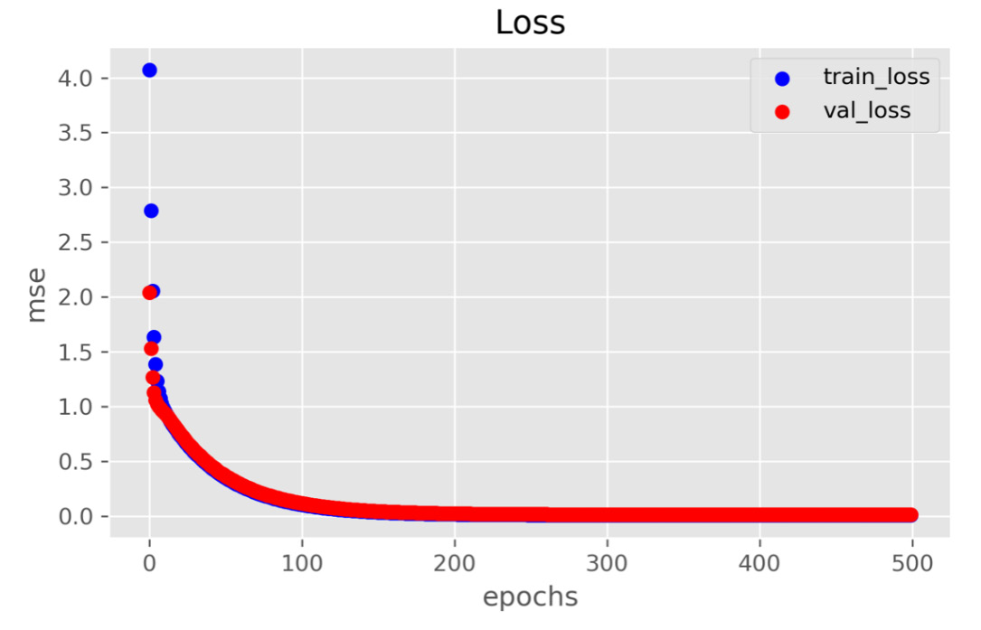
Figure 11.14: Minimizing the loss function by gradient descent

Similar to the process of minimizing loss in Exercise 11.01, Implementing a Gradient Descent Algorithm in NumPy, we see that both the training loss and validation loss are again dropping very quickly by the 100th epoch. After the 100th epoch, the loss starts to converge on a small number and becomes more and more stable.

This plot of training loss versus validation loss is a very telling visualization when training deep learning models. When we see both loss functions reduced to the minimum, this usually means 'the model is trained enough and has reached the best fit. If you continue to perform gradient descent after both loss functions reach the minimum, then you will overfit the model and you'll see that the validation loss starts to increase. This is when you need to stop training the model.

Note

To access the source code for this specific section, please refer to https://packt.live/30bU0t2.

In this exercise, we created a linear regression model using a PyTorch tensor with the requires_grad=True attribute. We then implemented the gradient descent algorithm using PyTorch's autograd package. Lastly, we visualized how loss functions behave during the training process and verified that our gradient descent algorithm had successfully trained the linear regression model.

So far, our gradient descent algorithm is using the whole training dataset at each epoch to calculate the gradient for all input data. This type of gradient descent is called batch gradient descent. "Batch" refers to the data for gradient computation as a whole batch. In practice, batch gradient descent isn't widely used in the real world. Instead, most industry practitioners use Stochastic Gradient Descent (SGD) or mini-batch Stochastic Gradient Descent (mini-batch SGD). We will discuss mini-batch SGD in-depth in the next topic.

Mini-Batch SGD with PyTorch

Let's recap what we have learned so far. We started by implementing a gradient descent algorithm in NumPy. Then we were introduced to PyTorch, a modern deep learning library. We implemented an improved version of the gradient descent algorithm in PyTorch in the last exercise. Now let's dig into more details about gradient descent.

There are three types of gradient descent algorithms:

• Batch gradient descent
• Stochastic gradient descent
• Mini-batch stochastic gradient descent

While batch gradient descent computes model parameter' gradients using the entire dataset, stochastic gradient descent computes model parameter' gradients using a single sample in the dataset. But using a single sample to compute gradients is very unreliable and the estimated gradients are extremely noisy. So, most applications of stochastic gradient descent use more than one sample, or a mini-batch of a handful of samples, to compute gradients; thus, this strategy is called mini-batch stochastic gradient descent.

You may wonder why most people use mini-batch SGD while batch gradient descent is rarely used. There are primarily two reasons why mini-batch SGD dominates over batch gradient descent in real-world practice:

1. Batch gradient descent is just simply too computationally expensive and the gain isn't justified by the huge computational cost.
2. A real-world model's loss function usually has many local minima. To escape local minima and find the global minima, the randomness in computing the gradient from a mini-batch can help the algorithm escape the local minima without getting trapped.

Let's dig into the deeper details of these points. The reason why batch gradient descent is too computationally expensive is that real-world datasets in the industry are usually web-scale and you won't be able to fit all of that data into a single machine. Imagine a company such as Google, which has billions of user searches per day – its data is easily at the scale of petabytes. Performing gradient calculations on data at such a scale is almost impossible.

Rather than computing the gradient using the whole dataset, mini-batch SGD randomly selects several samples from the dataset and calculates the gradient using these randomly selected samples. Because the computation cost is much reduced, mini-batch SGD is a lot faster than batch gradient descent:

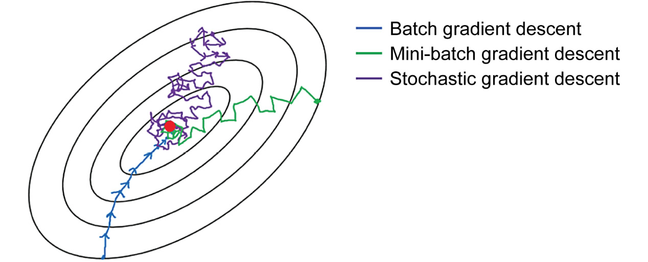
Figure 11.15: Comparison of different gradient descent algorithms

As the preceding figure suggests, batch gradient descent might get you the smoothest gradient descent path given all the data is being used, and mini-batch SGD is less optimal if significantly less data is used. SGD is expected to be the noisiest because it uses only one sample at a time. However, all of them can get you to the final destination – the global minima. Although the gradient estimated by mini-batch SGD is a little bit noisier than batch gradient descent and it takes a longer path to reach the minima, mini-batch SGD is still the preferred algorithm because of its computational advantage.

Having briefly discussed the problem of gradient descent, let's move onto another problem that is encountered in the loss functions of real-world datasets – multiple local minima. The loss function in a real-world deep learning model isn't always convex, nor does it always have a smooth path to the global minima. This results in the batch gradient descent algorithm getting trapped in the local minimum as illustrated in the following figure:

Figure 11.16: The algorithm gets trapped in the local minimum

One way to get the algorithm to escape the local minimum is to introduce some randomness in the gradient descent path so that it can be jerked out of the local minimum and land in a new region that leads to the global minimum:

Figure 11.17: Noise causes oscillations in the gradient descent path

As the preceding figure illustrates, batch gradient descent is more desirable in an ideal world where models have perfectly smooth convex loss functions. However, the oscillation behavior exhibited in mini-batch gradient descent is more desirable in reality, where models aren't perfectly convex, as they have multiple local minima.

Now let's implement a mini-batch SGD algorithm. Luckily, PyTorch has the utils module, which will help us tremendously in mini-batch SGD implementation. Besides this, we will also improve our model-building skills with best practices by using PyTorch's optim and nn modules.

Let's briefly introduce these submodules in PyTorch one by one:

• In the utils module, there is a data module, which contains many very handy helper functions that make passing data to the model very easy.
• The optim module implements various state-of-the-art optimization algorithms, including SGD. Instead of manually writing a gradient descent algorithm as we did in previous exercises, we will use the SGD algorithm implemented by the optim module in the next exercise.
• The nn module is the core module in PyTorch. It implements many high-level model abstractions over the concept of tensor. This means the classes in this module are built on top of tensor and extended with more methods and attributes.

We discussed that a deep learning model is made up of layers of tensors, which means we can implement different neural network models by putting tensor objects together in different ways, just like playing with Lego. The most Pythonic way of creating different models is through writing different classes that inherit from the same base class. In PyTorch, torch.nn.module is the base class for all neural network models. Essentially, a model in PyTorch is represented as a user-defined class that inherits from nn.module. If this sounds strange to you, we will show you some concrete examples in the next exercise.

Note

For more information about PyTorch, please visit its documentation at https://pytorch.org/docs/stable/index.html.

In the next exercise, we will implement mini-batch SGD in PyTorch with high-level modules such as the utils.data, optim, and nn modules.

Exercise 11.03: Implementing Mini-Batch SGD with PyTorch

In this exercise, we will improve the gradient descent algorithm by implementing mini-batch SGD with high-level PyTorch modules. We will still use a simple linear regression model as our baseline to implement the mini-batch SGD. At the highest level, most of the training procedure is still very similar to Exercise 11.01, Implementing a Gradient Descent Algorithm in NumPy and Exercise 11.02, Gradient Descent with PyTorch. But this exercise will require lots of code changes because we will be using high-level PyTorch modules for implementation instead of low-level tensor objects, as in Exercise 11.02, Gradient Descent with PyTorch.

To be more specific about what we need to do in this exercise, we will need to do the following:

1. We will use the utils.data module to create data loader objects for generating mini-batches in the training procedure.
2. We will implement our simple linear regression model by defining a model class that inherits from nn.module.
3. We will implement mini-batch SGD using the optim module.

Perform the following steps to complete the exercise:

1. In the Chapter11 directory, launch a Jupyter Notebook in your Terminal (macOS or Linux) or Command Prompt window (Windows).
2. After the Jupyter Notebook is launched, create a new directory named Exercise11.03. Inside the Exercise11.03 directory, let's create a Python 3 notebook.
3. Inside the Python3 notebook, import all the necessary modules as shown in the following snippet:

   # import modules

   import numpy as np

   import torch

   import torch.optim as optim

   import torch.nn as nn

   from torch.utils.data import DataLoader,

        TensorDataset, random_split

   import matplotlib.pyplot as plt

   plt.style.use('ggplot')

   device = 'cuda' if torch.cuda.is_available() else 'cpu'

   In addition to numpy and matplotlib, we import torch.optim for SGD, torch.nn for creating the linear regression model, and torch.utils.data for feeding batches into the model.

4. Generate some syntactic data using numpy for the linear regression model as shown in the following code:

   # set random seed

   np.random.seed(9)

   # draw 100 random numbers from uniform dist [0, 1]

   x = np.random.uniform(0, 1, (100, 1))

   # draw random noise from standard normal

   z = np.random.normal(0, .1, (100, 1))

   # create ground truth for y = 8x - 3

   y = 3 * x - 1 + z

5. After the data is generated, we will convert the data from the form of numpy to the form of TensorDataset as shown in the following code:

   # move data from numpy to torch

   x_tensor = torch.from_numpy(x).float().to(device)

   y_tensor = torch.from_numpy(y).float().to(device)

   # create tensor dataset from tensor

   dataset = TensorDataset(x_tensor, y_tensor)

   print(dataset[0])

   You should get the following output:

   (tensor([0.0104]), tensor([-1.0155]))

   You will notice that TensorDataset() is very similar to the Python built-in function zip(). It takes as input *tensors (1 tensor or more) and retrieves the nth sample from *tensors to bundle them into a tuple so that the nth sample from *tensors can be retrieved by indexing. In the output, we see that tensor([0.0104]) is the first sample x_tensor and tensor([-1.0155]) is the first sample y_tensor.

   The reason why we convert our data to TensorDataset() is because torch.utils.data helper functions are expecting input data in the form of TensorDataset and not any other form. In the next step, you will see how we can create DataLoader out of TensorDataset.

6. Now let's create DataLoader for the training and validation datasets, as shown in the following code:

   # split data into train and eval

   train_dataset, val_dataset = random_split(dataset, [80, 20])

   # create data loader

   train_loader = DataLoader(dataset=train_dataset, batch_size=8)

   val_loader = DataLoader(dataset=val_dataset, batch_size=10)

   Notice that we use the random_split helper function from the torch.utils.data module to split the data with a ratio of 80 to 20 for the training and validation datasets. Both train_dataset and val_dataset are still in the form of TensorDataset.

   Then we create DataLoader for both train_dataset and val_dataset with batch sizes of 8 and 10 respectively. The batch size of 8 for the training data loader means it will generate 8 randomly selected samples from the training dataset every time it gets invoked.

   The batch size for the validation data loader doesn't have to be the same as the one for the training data loader. The batch size for the training data loader could impact our mini-batch SGD's performance. For the validation data loader, the batch size can be an arbitrary number. It does not impact the mini-batch SGD. If the whole validation dataset can fit into RAM, then you can set its batch size as the size of the whole validation dataset.

7. Next, we will define our linear regression model by creating a Python class that inherits from nn.Module as shown in the following code:

   # define our linear regression model in pytorch

   class LinearRegression(nn.Module):

       def __init__(self):

           super().__init__()

           self.linear = nn.Linear(1, 1)

       def forward(self, x):

           return self.linear(x)

   # initialize our model

   model = LinearRegression().to(device)

   # state_dict() contains the parameters of the model

   print(model.state_dict())

   To create a model class in PyTorch, you need to implement an __init__(self) constructor and the forward(self, x) method. In the constructor, you will initialize attributes for the model class. Notice that the only attribute is nn.Linear(1,1), which is also a model class that inherits from nn.Module. The nn.Linear(1,1) object is another nn.Module. It's a generalized form of a linear model that applies a linear transformation to its input data. In this case, we specify (1,1). This means the linear model will map a piece of one-dimensional input data to another piece of one-dimensional output data. It is equivalent to a simple linear regression, y = bias + weight * x.

   The other important method you have to implement is forward(self, x). This defines the forward pass for the model. In our case, the model applies a linear transformation for an input, x, and returns the transformed value, which is y_hat = bias + weight * x.

8. Next, we will create a loss function from the torch.nn module and the SGD optimization algorithm from the torch.optim module as shown in the following code:

   # set training routine

   lr = 1e-1

   n_epochs = 50

   # create loss function and optimizer

   loss_fn = nn.MSELoss(reduction='mean')

   optimizer = optim.SGD(model.parameters(), lr=lr)

   We set the learning rate to 0.1 and number of epochs to 50. Our loss function is still MSE. PyTorch provides a variety of loss functions in the torch.nn module, so we don't have to manually derive the loss function from the input data.

   Our optimizer is optim.SGD, which is a standard SGD algorithm. To create one, you need to pass in the model's parameters (weight and bias), which can be accessed via the .parameters() method, and the learning rate. In the next step, you will see how we create a gradient descent algorithm using the loss function and an optimizer.

9. We will define a function that performs the mini-batch SGD as shown in the following code:

   def train_one_batch(model, loss_fn, optimizer, x_batch, y_batch):

       model.train()

       # forward pass

       yhat = model(x_batch)

       # calculate training loss

       loss = loss_fn(y_batch, yhat)

       # gradient descend

       loss.backward()

       optimizer.step()

       optimizer.zero_grad()

       return loss.item()

   Let's go through the preceding code line by line. The first line, model.train(), is a bit misleading the first time you see it. This method call does not train the model. Instead, it just sets the model in training mode. The next line performs the forward pass and outputs the model predictions for the small batch of input data. Then we use the loss function we defined in the previous step to calculate the MSE loss. The next three lines take care of gradient descent. The loss.backward() function performs backpropagation to calculate the gradients for the model parameters. The optimizer.step() function performs a parameter update, which subtracts the parameter value from the learning rate * gradient. The last line, optimizer.zero_grad(), zeroes out all of the cached gradients in the computational graph.

10. Next, we will actually start the model training procedure as shown in following code:

    # train model

    losses = []

    val_losses = []

    for epoch in range(n_epochs):

        print("[ epoch ]", epoch)

        tmp_losses = []

        for idx, (x_batch, y_batch) in enumerate(train_loader, 1):

            x_batch = x_batch.to(device)

            y_batch = y_batch.to(device)

            loss = train_one_batch(model, loss_fn, optimizer,

                                   x_batch, y_batch)

            tmp_losses.append(loss)

        print("[ training ] training loss = {}"

              .format(sum(tmp_losses)/idx))

        losses.append(sum(tmp_losses)/idx)

        # eval

        with torch.no_grad():

            # set eval mode

            model.eval()

            tmp_val_losses = []

            for idx, (x_batch, y_batch)

                      in enumerate(val_loader, 1):

                x_batch = x_batch.to(device)

                y_batch = y_batch.to(device)

                yhat = model(x_batch)

                tmp_val_losses.append(loss_fn(y_batch, yhat)

                                      .item())

            print("[ eval ] validation loss = {}"

                  .format(sum(tmp_val_losses)/idx))

            val_losses.append(sum(tmp_val_losses)/idx)

            

    print(model.state_dict())

    You should get the following output:

    

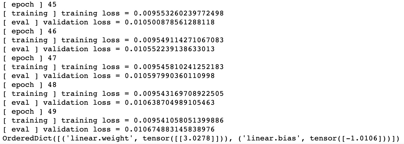
    Figure 11.18: Logs of the model training process

    Note

    We will have loads of output data with 500 iteration results. We have only shown the last section of it in the preceding figure.

    This step is somewhat similar to Step 8 in Exercise 11.02, Gradient Descent with PyTorch. The biggest difference is that we are implementing mini-batch SGD in this exercise. For each epoch, the algorithm generates (x_batch, y_batch) from train_loader. Recall how in Step 6, we set the batch size for the training data loader to be 8, so it will generate 8 samples for each iteration. The heavy-lifting work for model training is done by the train_one_batch function, which was defined in the previous step. The remaining logic in this snippet mostly records training losses and validation losses for later visualization.

11. Finally, let's visualize how the MSE loss function is minimized during the gradient descent as shown in the following code:

    plt.scatter(range(n_epochs), losses, label='train_loss',

                color='b')

    plt.scatter(range(n_epochs), val_losses, label='val_loss',

                color='r')

    plt.legend()

    plt.title('Loss')

    plt.xlabel('epochs')

    plt.ylabel('mse')

    plt.tight_layout()

    You should get the following output:

    

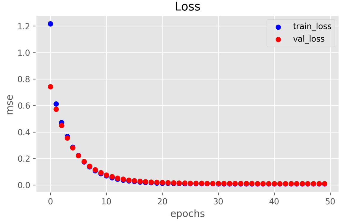
Figure 11.19: Minimizing the loss function with mini-batch SGD

You may notice that it only took 28 epochs to converge in mini-batch SGD, compared to over 100 epochs in batch gradient descent. This is because there are more iterations in each epoch in mini-batch SGD compared to the one iteration in each epoch in batch gradient descent. The number of iterations in each epoch equals the number of samples in the training dataset divided by the number of samples in the mini-batch.

Note

To access the source code for this specific section, please refer to https://packt.live/2C7VCMw.

In this exercise, we learned that mini-batch SGD is a better algorithm in the real world than batch gradient descent. To implement mini-batch SGD, we leveraged PyTorch's high-level abstractions, such as torch.nn for creating the model class, torch.utils.data for creating the data loader, and torch.optim for SGD optimization.

So far, we've covered both the theoretical part and the practical part of developing and training machine learning models. For the theoretical part, we learned the core concepts in neural networks such as constructing the loss function for your model and minimizing the loss function via the gradient descent approach. For the practical part, we learned to build and train models in both NumPy and PyTorch. Now that we have the theory and practical skills in machine learning modeling, we are ready to explore a more interesting field in machine learning: reinforcement learning.

We will discuss and implement a reinforcement learning algorithm in the next section.

Building a Reinforcement Learning Algorithm to Play a Game

One of the very important breakthroughs in the AI community happened in 2016 when a computer program called AlphaGo outplayed the best human professional Go player at the board game Go. This breakthrough shook the world and triggered tremendous hype around AI not only in academia but also in various industries.

The AlphaGo algorithm is an example of a reinforcement learning algorithm. Reinforcement learning is very different from supervised learning. The simple linear regression model from our previous exercises is an example of supervised learning. In previous exercises, we provided the training algorithm with training data input, x, and an output, y. After several epochs of parameter updates, the training algorithm could find estimates for the weight and bias that were extremely close to the ground truth. As you can see, the objective of supervised learning is to minimize the distance between the model's estimate and the ground truth.

Unlike supervised learning, there is no ground truth in reinforcement learning. Imagine you are playing the game of Go. You and your opponent take turns to place a stone on the board at each step. You and your opponent are trying to control the territory by making a boundary to capture one another's stones. Go is a strategy game. There are many ways to win and each way of winning also depends on the moves your opponent has made. When you are playing a strategy game, you are dealing with uncertainty at the present moment, but you know there is a path to winning. Supervised learning requires certainty and ground truth, which is not available in this case, so we will need a new approach to solve this kind of problem. For representational purposes, you can get an idea of the game Go from the following figure:

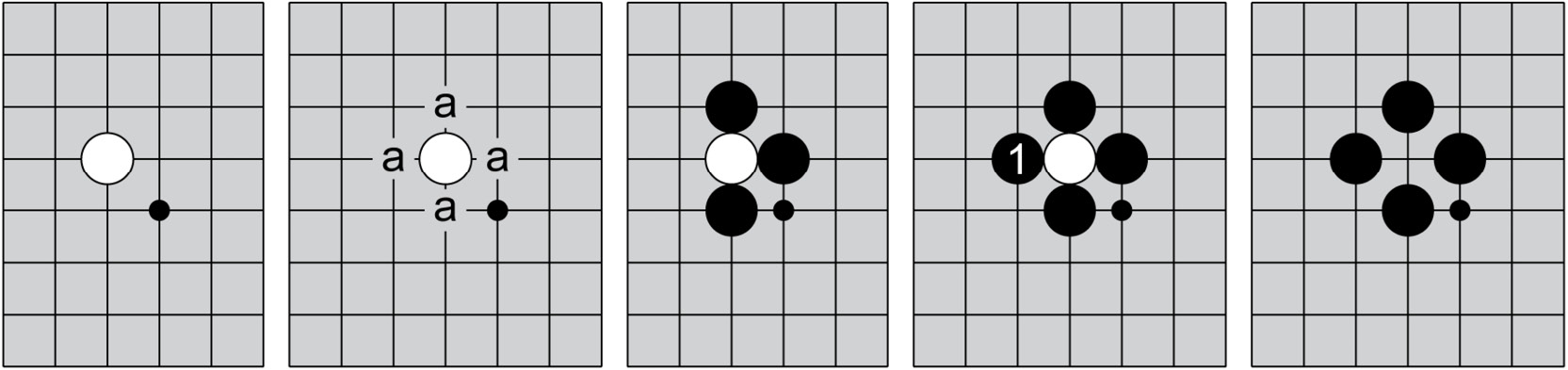
Figure 11.20: The game Go

Reinforcement learning trains an agent that tries to maximize some notion of reward by taking a series of "best" actions given a series of corresponding environment states. When playing Go, every time your opponent makes a move, the state of the board with black and white stones in different positions is a new environment state. Based on the given environment, the agent needs to find an optimal action that will eventually lead to a maximum reward:

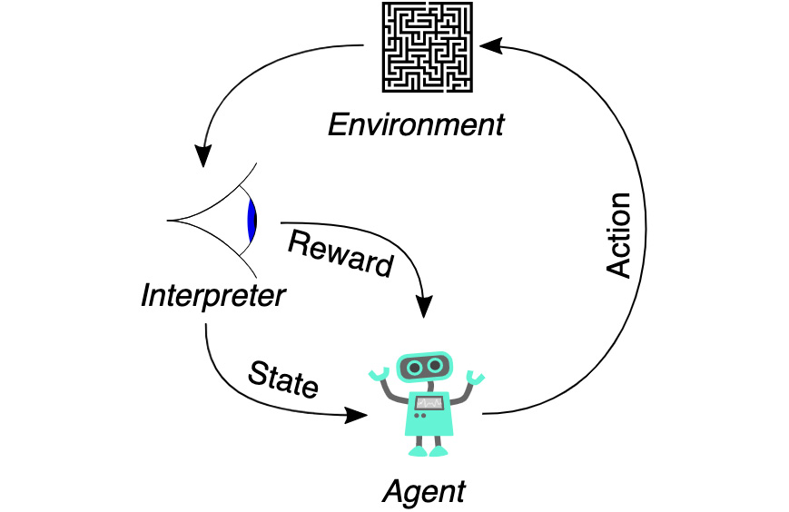
Figure 11.21: Overview of the reinforcement learning algorithm

The preceding figure illustrates all of the components in reinforcement learning. Let's use the board game Go as an example. The Agent, or in our case the algorithm, is the player. The Agent is trained to make a "best" Action, which means placing a stone in a position on the board such that the agent's chances of winning the game are maximized. After the Agent places a stone, the opponent player will also make a move. Now the board is changed by two new stones being placed in different positions, which means the Environment is changed. The next Action is for the Agent to learn from the past. However, the Agent is a computer algorithm. We need to feed the algorithm with data that the computer can understand and digest. So, we need an Interpreter. The Interpreter needs to accomplish two things. One is to interpret Reward in terms of a score. The other one is translating an Environment into a State, which should be an array of real numbers and can be digested by a computer algorithm. Now the Agent can learn to improve from the past by looking at the past states and rewards. Finally, the Agent will make the "best" action again for the given state and the cycle starts over again.

Now let's dig deeper into how the agent learns to improve its game. As the board game Go is being played, the agent records the state and the reward for every iteration so that the agent can learn as they play the game. During its learning time, the agent retrieves a batch of states and rewards from its memory and tries to come up with a policy that can tell it the reward of different actions so that it can pick the action that maximizes the reward. However, the policy is far from being accurate at the beginning of the game. As the game goes on, the policy will improve and make a more accurate prediction for the reward. This is where exploration versus exploitation comes into place. The longer the agent explores, the more the policy can learn. However, the returns of excessive learning will diminish eventually. So, the agent needs to start to exploit the policy after the agent starts to trust the policy. The strategy for trading off between exploration and exploitation is called an epsilon-greedy strategy:

Figure 11.22: Epsilon-greedy policy

Basically, for every iteration, the agent can either take a random action (or "arm") or listen to the policy and make the "best" action that maximizes the reward. To determine which way to go, we will draw a random number from a uniform distribution and compare the random number to the value of epsilon. The value of epsilon and the probability of choosing the random action will decay exponentially as the game goes on. This means the agent gradually leans toward the policy and converges on the policy eventually.

You may wonder how the policy can predict the reward for a given state and choose an action. Let's start with a simple game such as Tic-Tac-Toe. The reward for this game is either a win (+1), a loss (-1), or a draw (0). Depending on which player starts first, you can write a simple computer program to perfectly play the game to not lose. This is because the game's state-space complexity is very small and has a total of 765 different positions. Mathematically speaking, all 765 different states can be represented in the form of a Markov decision process (MDP), which is like a tree where the next state depends on the development of previous states:

Figure 11.23: MDP for Tic-Tac-Toe

As the game tree in the preceding figure illustrates, the space of the states in the game is finite. This means there is always a path of a given state and a chosen action that leads to the ultimate reward. This is our policy – the agent will look at the policy and find out which action leads to a win and it will take that action.

Note

You can refer to the following link to find out more about MDPs:

http://www.pitt.edu/~schaefer/papers/MDPTutorial.pdf

For a game like Go, the state space is infinite and unbounded. Its MDP is too large to be represented by an exact mathematical model. This is where neural networks come in handy. We can train a neural network to approximate the game's MDP. The neural network will predict the reward given a state and an action. Note that the reward is a cumulative reward, which is represented by in the following equation:

Figure 11.24: Formula of the cumulative reward

The cumulative reward is the sum of future discounted rewards for each timestamp, t. The symbol ɣ is a discounted factor with a value between 0 and 1. In the game of Tic-Tac-Toe, the cumulative reward at the end of the game is +1 if we win, -1 if we lose, or 0 if it's a draw. The reward for each step could be different for different games. The definition of a reward for each step is usually up to us to define. In the game of Tic-Tac-Toe, it would be a fraction of 1. To make the math work, the reward decays exponentially into the future so that the sum will converge on a finite value that is predictable by the neural network. Also, the discounted factor makes the neural network biased toward recent rewards. The action that the agent takes at the current moment has far more impact on the cumulative reward than the actions deep in the future. Just like playing a game of Tic-Tac-Toe, the location you choose to draw an O at the current moment will directly impact where your opponent will draw an X because your opponent tries to read what you are doing and stop you from winning the game.

This cumulative reward is also known as the Q value in the reinforcement learning paradigm. The neural network that approximates the MDP is the Q-function, also known as a deep Q neural network. In summary, the process in which the neural network is trained to better approximate the Q value is called deep Q-learning:

Figure 11.25: Take the best action that maximizes the Q value

The Q function predicts the Q value for a given state and action. The agent will choose the action that maximizes the Q value and the ᴫ* symbol represents the best action for the given state. Imagine that when playing the game of Tic-Tac-Toe, drawing an O at the center at the start of the game will maximize the chance of winning, thus maximizing the Q value.

So far, we still don't know what exactly the Q function is, in just the same way as the agent doesn't know how to play the game to win. However, the Q function always obeys the Bellman equation, shown in the following formula:

Figure 11.26: Bellman equation

This formula says the approximated Q value at the current step with state=s and action=a is equal to the current reward plus a discount factor ɣ weighted Q value at the next step (state=s'). We can use this Bellman equation to construct the loss function for the Q function as shown in the following formula. In the example of Tic-Tac-Toe, it means we can use the current reward plus the predicted cumulative reward at the next step to approximate the cumulative reward for the current step:

Figure 11.27: Loss function of the Q-learning algorithm

After the loss function is defined, we can use what we learned in previous exercises to perform gradient descent to find out the best fit for the Q function and use the Q function as our policy to play the game to win.

Now that we've learned the basic theory behind reinforcement learning, it's time to apply it to a problem. In the next exercise, we will implement a reinforcement learning algorithm to play the game of CartPole-v1 from OpenAI Gym.

Exercise 11.04: Implementing a Deep Q-Learning Algorithm in PyTorch to Solve the Classic Cart Pole Problem

In this exercise, we will play the game of CartPole-v1. It's a classic control theory problem where the goal is to balance a pole attached to a cart on a frictionless track. A representation of the game is shown in the following figure:

Figure 11.28: Balancing the cart pole from OpenAI Gym

While playing the game, the agent can apply a force of +1 or -1 to the cart to help the pole remain balanced. A reward of +1 is provided for each timestep that the pole remains balanced for. For more details about this game, please visit https://gym.openai.com/envs/CartPole-v1/.

Before proceeding to the exercise, please make sure you have installed the Gym. If you haven't installed it, please follow the installation instructions in the Preface.

Perform the following steps to complete the exercise.

1. In the Chapter11 directory, launch a Jupyter Notebook in your Terminal (macOS or Linux) or Command Prompt window (Windows).
2. After the Jupyter Notebook is launched, create a new directory named Exercise11.04. Inside the Exercise11.04 directory, create a Python 3 notebook.
3. Inside the Python 3 notebook, import all the necessary modules and seed the environment as shown in the following code block:

   # import module

   import random

   import numpy as np

   from itertools import count

   from collections import deque

   import torch

   import torch.nn as nn

   import torch.nn.functional as F

   import torch.optim as optim

   import gym

   # make game

   env = gym.make('CartPole-v1')

   # seed the experiment

   env.seed(9)

   np.random.seed(9)

   random.seed(9)

   torch.manual_seed(9)

   The env = gym.make('CartPole-v1') line creates the cart pole game for this exercise. In the last four lines in the snippet, we seed the randomness for those four libraries that we will use in later steps.

4. Let's define our deep Q network (DQN) as shown in the following code:

   # define our policy

   class DQN(nn.Module):

       def __init__(self, observation_space, action_space):

           super(DQN, self).__init__()

           self.observation_space = observation_space

           self.action_space = action_space

           self.fc1 = nn.Linear(self.observation_space, 32)

           self.fc2 = nn.Linear(32, 16)

           self.fc3 = nn.Linear(16, self.action_space)

       def forward(self, x):

           x = F.relu(self.fc1(x))

           x = F.relu(self.fc2(x))

           x = self.fc3(x)

           return x

   We define a class called DQN, which is a simple three-layer feedforward neural network model with rectified linear unit (ReLU) activation functions in between each layer. ReLU activation is commonly found in modern neural network architectures.

   The DQN takes an input state with four features (for example, tensor([1,0,1,0])) and output the Q values (for example, tensor([1.2, 0.4])) for the action of left force (-1) and the action of right force (+1). The input state with four features describes the position and angle of the cart pole in the game. For the moment, we don't need to understand what each of the numbers means. The algorithm will figure out a way to learn the better action (either a left force or a right force) for a given input state such that the cart pole remains in a balanced state. This is the magic part of machine learning.

5. Next, we will create the agent to play the game as shown in the following code:

   ex04-notebook.ipynb

   # define our agent

   class Agent:

       def __init__(self, policy_net):

           MEMORY_SIZE = 10000

           GAMMA = 0.6

           BATCH_SIZE = 128

           EXPLORATION_MAX = 0.9

           EXPLORATION_MIN = 0.05

           EXPLORATION_DECAY = 0.95

           self.policy_net = policy_net

           self.optimizer = optim.RMSprop(

                            policy_net.parameters(), lr=1e-3)

           self.memory = deque(maxlen=MEMORY_SIZE)

           self.gamma = GAMMA

           self.batch_size = BATCH_SIZE

           self.exploration_rate = EXPLORATION_MAX

           self.exploration_min = EXPLORATION_MIN

           self.exploration_decay = EXPLORATION_DECAY

       

       def select_action(self, state):

           if np.random.rand() < self.exploration_rate:

               return torch.tensor([[random.randrange(

                                   self.policy_net.action_space)]])

           else:

               with torch.no_grad():

                   q_values = self.policy_net(state)

               return q_values.max(1)[1].view(1,1)

   The full code is available at https://packt.live/2Wh0hTo.

   Notice we implemented three methods for the Agent class: select_action(), remember(), and experience_replay(). These three methods describe the responsibility of the agent. The agent needs to take action – remember that the game is played in light of the outcome – and learn to play the game better.

   At each timestamp, the agent is responsible for choosing the "best" action (left force or right force) to keep the pole balanced. Recall the concept of the epsilon-greedy strategy for tackling the challenge of exploration versus exploitation. self.exploration_rate is the epsilon, which starts its value at EXPLORATION_MAX=0.9 and will decay over time with a factor of EXPLORATION_DECAY=0.95 until it reaches its minimum value at EXPLORATION_MIN = 0.05.

   While playing the game, the agent also needs to record past actions and states for training the DQN model. The remember() method is called to record the state, action, reward, and the next state for every timestep during the game.

   The experience_replay() method is used to train our DQN policy for every timestamp. It first draws samples from previous timestamps during the game. It then makes two different forward passes to get Q values and expected Q values. Recall the following loss function:

   

   Figure 11.29: Loss function of the Q-learning algorithm

   The first term in the equation, , is calculating the actual Q values from states and their corresponding actions. The second term in the equation, 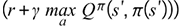, is calculating the expected Q values using the optimal actions and their corresponding next states.

   Lastly, we use F.smooth_l1_loss to calculate the loss function. This loss function is the Huber loss function, which is also very commonly used in training DQNs.

   After gradient descent for this learning round is completed, we update the epsilon self.exploration_rate to make sure it decays exponentially to the minimum value.

6. Finally, we will implement the deep Q-learning training loop as shown in the following code:

   ex04-notebook.ipynb

   # create policy

   observation_space = env.observation_space.shape[0]

   action_space = env.action_space.n

   policy_net = DQN(observation_space, action_space)

   # create agent

   agent = Agent(policy_net)

   # play game

   game_durations = []

   for i_episode in count(1):

       state = env.reset()

       state = torch.tensor([state]).float()

       print("[ episode {} ] state={}"

             .format(i_episode, state))

       for t in range(1, 10000):

           action = agent.select_action(state)

           state_next, reward, done, _ = env.step(action.item())

           if done:

               state_next = None

           else:

               state_next = torch.tensor([state_next]).float()

           agent.remember(state, action,

           torch.tensor([[reward]]).float(), state_next)

           print("[ episode {} ][ timestamp {} ] state={},

                 action={}, reward={}, next_state={}"

                 .format(i_episode, t, state, action,

                         reward, state_next))

   The full code is available at https://packt.live/2Wh0hTo.

   Before the training loop starts, we initialize the policy and agent. In the main training loop, the game environment is reset for each episode. An episode ends if the pole loses balance and falls over. For each timestep in an episode, the agent will select an action based on the epsilon-greedy strategy and execute it. After the action is taken, the game returns the reward and new states. The agent will put the information into its memory, as well as executing an experience replay to optimize the policy.

   For the lines at the bottom of the previous snippet, we limit the main training loop to 500 episodes. If there's confusion between the concepts of an episode and an epoch, an epoch is a concept for gradient descent whereas an episode is a concept in playing games. An episode means playing a game through once. 500 episodes means playing a game 500 times.

   If the agent requires more than 500 episodes to converge, then this is not a good deep Q-learning algorithm and it is failing to converge. If the agent can last long enough with the number of timesteps greater than env.spec.reward_threshold, which is set to 500 timesteps, in an episode, then the agent wins the game.

   After you have run the training loop, you should get the following output:

   

   Figure 11.30: Output logs of the main training loop

   Note

   We will have loads of output data with 500 iteration results. We have only shown the last section of it in the preceding figure.

   The output tells us that the agent can keep the pole balanced for 500 timesteps at episode 184. According to the game's reward spec, this is a winning solution.

7. Lastly, let's visualize how our deep Q-learning algorithm improves over time by running the following code:

   import matplotlib.pyplot as plt

   plt.style.use('ggplot')

   plt.scatter(range(i_episode), game_durations)

   plt.title('Game Duration Over Time')

   plt.xlabel('game episode')

   plt.ylabel('game duration')

   plt.tight_layout()

   You should get the following output:

   

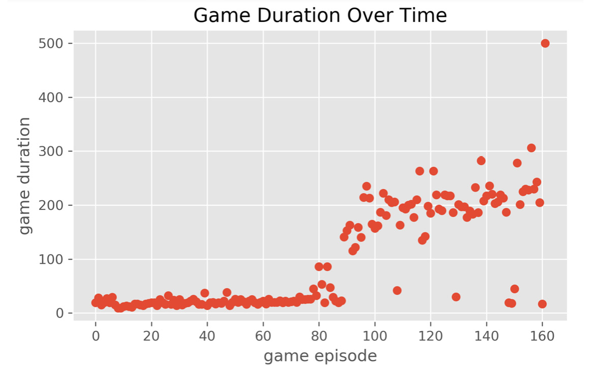
Figure 11.31: Game duration increases to 500 after 175 episodes

We can see that our deep Q-learning algorithm learns to keep the pole balanced for longer and longer as the number of episodes increases. During the first 80 episodes, our model learns very slowly, then it suddenly makes a huge improvement between the 80th and 120th episodes. However, after the 120th episode, the algorithm fails to continue to converge and isn't able to keep the pole balanced for long. After the 160th episode, the algorithm gets back on track and converges on a solution and keeps the pole balanced for more than 500 timestamps. The pattern of convergence is also a result of the epsilon-greedy strategy. Recall the concept of exploration and exploitation: for the first 80 episodes, the algorithm wasn't able to take good actions to keep the pole balanced. This is because the algorithm spent more time on exploration than on exploiting its policy. Later, as its policy improved, the algorithm started to exploit more and explore less. Therefore, we see a convergence after 90 episodes.

Note

To access the source code for this specific section, please refer to https://packt.live/2Wh0hTo.

Let's recap what we learned in this exercise. We started it by learning the math and theory behind reinforcement learning for playing a game, looking in particular at the deep Q-learning algorithm. We then went on to implement the deep Q-learning algorithm to play CartPole-v1 from OpenAI Gym. We first defined the DQN model, then we created an agent that implemented an epsilon-greedy strategy and experience replays for model training. We then coded up the main training loop for optimizing our deep Q-learning algorithm. Lastly, we visualized how the algorithm improved over time.

Notice in Figure 11.31 that our deep Q-learning algorithm doesn't converge consistently. The number of timesteps in one episode fluctuates up and down wildly between the 125th episode and 175th episode. This is probably when the model is overfitting the Q values for actions during that time. We used the same DQN for calculating both the Q values and the expected Q values. The loss from the same function sometimes doesn't converge well, which results in the model overestimating the Q values. The natural question is this: can we improve the algorithm to stabilize the loss function?

The answer is yes. In 2015, Hado van Hasselt, along with two other scientists, proposed a new reinforcement learning algorithm: double Q-learning. The idea behind double Q-learning is simple. Because using the same DQN to calculate the loss is problematic, we can use two different DQN models: one is for action selection, and the other one is for calculating the expected Q values. We call the first one a policy neural network and the second one the target neural network. For more information about double Q-learning, please refer to https://arxiv.org/abs/1509.06461.

In the next activity, we will take what we have learned from this chapter, particularly from the last exercise, and apply it. We will implement a double deep Q-learning algorithm to play CartPole-v1 from OpenAI Gym.

Activity 11.01: Implementing a Double Deep Q-Learning Algorithm to Solve the Cart Pole Problem

In this activity, we will implement a double deep Q-learning algorithm for the cart pole problem. Recall how in Exercise 11.04, Implementing a Deep Q-Learning Algorithm in PyTorch to Solve the Classic Cart Pole Problem, we used a single DQN model to calculate the Q-learning loss function. In this activity, we will use two DQN models to calculate the Q-learning loss function. In particular, one DQN will be used for choosing the best action, which is called the policy network. The other DQN will be used for estimating the expected Q value for a given state, which is called the target network.

The reason why we chose to play the same game is that we can compare the two different algorithms at the end of the game with all else being equal. The rules are the same as for the previous exercise.

Note

The code and the resulting output for this exercise have been loaded in a Jupyter Notebook that can be found here: https://packt.live/2OzZOrb.

Perform the following steps to complete the activity:

1. Import all necessary modules, such as numpy, torch, gym, matplotlib.pyplot, and others. Don't forget to set the seed for all the random number generators that will be used in later steps.
2. Define the model architecture for the DQN for both policy_network and target_network, which are two different model instances using the same model architecture.
3. Create an agent that implements three methods: select_action(), remember(), and experience_replay(). In the experience_replay() method, please use policy_network to calculate the Q values while using target_network to calculate the expected Q values.
4. Implement the training loop for the double deep Q-learning algorithm. The training loop is similar to the one in the previous exercise. The only difference is that you need to implement the loss function with two DQNs, the policy network, and the target network. The output of the training loop should look similar to the following:
   

   Figure 11.32: Output logs of the main training loop

   Note

   We will have loads of output data with 500 iteration results. We have only shown the last section of it in the preceding figure.

5. Lastly, create a plot to visualize the algorithm's improvement over the episodes. The plot should look similar to the following:
   

Figure 11.33: Game duration increases to 500 after 133 episodes

With a double Q-learning algorithm, the algorithm can converge faster and in a more consistent fashion.

Note

The solution to this activity can be found on page 649.

Summary

This chapter gave you an overview of the theory underpinning machine learning algorithms, looking at constructing a loss function, and using gradient descent. These fundamental concepts will help you better understand a lot of the implementation details of current deep learning practices. They will also help you separate yourself from your peers. The exercises in this chapter focused on hands-on practical skills such as building and training machine learning algorithms for AI from scratch. With the practical skills you learned from this chapter, you will be able to build machine learning models to solve real-world problems.

We started by training a simple linear regression model and implementing a gradient descent algorithm using NumPy from scratch, which helped us better understand how to train a machine learning model. Then we moved on to building training models with PyTorch low-level modules. We also talk about batch gradient descent versus mini-batch SGD in depth. We then implemented mini-batch SGD using high-level PyTorch modules such as torch.nn, torch.optim, and torch.utils. At the end of the chapter, we introduced deep Q-learning and double deep Q-learning for reinforcement learning. We also implemented both of these learning algorithms to play the cart pole game from OpenAI Gym. With all of the hands-on practical skills we gained from this chapter's exercises, we are ready to solve more interesting problems in the world of machine learning.

In the next chapter, you will continue to build on your machine learning knowledge and enhance your understanding of AI infrastructure concepts, as well as developing the practical skills you learned in the previous chapters. You will be learning how to build a production-level AI application.