In this chapter, we’ll tie a lot of things together that we have covered in the book. The end goal of an AI application should always be to bring business value. That means all the great models that are created by data scientists should be put into production. It’s quite difficult to productionize and maintain an application that contains one or more machine learning models. In this chapter, we’ll discuss three major options for productionizing an AI application, so you’ll be well equipped to pick a method for your situation.
By the end of this chapter, you will be able to describe the steps it takes to run a machine learning model in production, list a few common options to run models in production, and design and implement a continuous delivery pipeline for models.
Introduction
In the previous chapters, you have learned ways to set up a data storage environment for AI. In this chapter, we will explore the final step: taking machine learning models into production, so that they can be used in live business applications. There are several methods for productionizing models, and we will elaborate on a few common ones.
Data scientists are trained to wrangle data, pick a machine learning algorithm, do feature engineering, and optimize the models they create. But even an excellent model has no value if it only runs in a machine learning environment or on the laptop of the data scientist; it has to be deployed in a production application. Furthermore, models have to be regularly updated to reflect the latest feedback from customers. Ideally, a model is continuously and automatically refreshed in a feedback loop; we call that reinforcement learning. An example of a system that uses reinforcement learning is a recommendation engine on a video website. Every time the algorithm makes a recommendation to a customer to view a movie, it tracks whether the recommendation is followed. If that is the case, the connection between the customer profile (the features of the algorithm) and the recommendation becomes stronger (reinforced), making a similar recommendation more likely in the future.
At this moment, it’s important to realize that models don’t have to run in an API, a data stream, or in an interactive way at all. It’s perfectly acceptable to run a model periodically (say, once per day or even once per month) on a dataset, and write the outcomes to a lookup table. In this way, data is preselected to be used by a live application. A production system only has to find the right records with a simple query on the lookup table. However, more and more systems rely on model execution on demand, simply because the results have to be updated in real-time.
In this chapter, we will describe a few options for running models in production. First, we’ll look at ways to export a model from a machine learning environment to run it in production. A common approach is to serialize a model into an intermediate format such as pickle and load the resulting files in an API. In this way, your model functions as the core functionality in a microservice.
Next, we’ll look at the most popular framework for running containers: Docker. Based on this framework, all public cloud providers offer scalable services that allow customers to run their containers with ease. Kubernetes, OpenShift, and Docker Swarm are examples of services that make use of Docker images.
Finally, we’ll describe a method to run models in a streaming data environment. Since performance is an important requirement for streaming data engines, we have to keep the latency low by making our model execution as effective as possible. This can be done by loading the models into an in-memory cache with an intermediate format such as PMML.
Let’s start with a basic form of serving models in production: creating an API. We will use the popular frameworks pickle and Flask for this.
pickle and Flask
A machine learning model can “live” in (be part of) many different environments. The choice of environment should depend on the type of application that is being developed, the performance requirements, and the expected frequency of updates. For example, a model that has to predict the weather once per day for a weather analyst has different requirements than a model that makes friend suggestions for millions of people on a social network.
For extreme cases, there are specialized techniques such as streaming models. We’ll have a look at them later in this chapter. For now, we’ll focus on a method that works for most use cases: running a model as part of an API. In doing so, our model can be part of a microservices architecture, which gives a lot of flexibility and scalability. To build such an API, pickle and joblib are two popular libraries that can be used when working with Python models. They offer the possibility to capture a dataset or a model that was trained in memory, thereby preparing it for transportation to a different environment. As such, this is a good way to share the same model in the development, testing, and production environments. There are also some disadvantages. pickle and joblib are not language-neutral since they can only be used in Python environments. This gives both data scientists and data engineers a disadvantage since it would be better to have a wider set of technologies to choose from. If you require a cross-platform framework, you could be better off with (for example) Express.js, Spring Boot, or FastAPI for API development and PMML or PFA for model serialization. However, if you’re sure that both the machine learning environment and the production environment are running Python, pickle and joblib are good options for serializing your models. They are well documented, easy to use, high performing, and have a large customer base and community behind them.
We will focus in the first exercise of this chapter on the pickle framework. You will learn how to serialize (or pickle) a simple model, and how to unserialize or marshal (unpickle) it. Serializing is the process of exporting a model that is built in a notebook. The model lives in the memory of a server in a file format such as JSON, XML, or a binary format. A serialized model can be treated like any other asset in an application; this is needed to transport the model, create versions of it, and deploy it. Then, you will use the model in a Flask API to execute it and get predictions from an input dataset. Let’s implement this in the next exercise.
Exercise 12.01: Creating a Machine Learning Model API with pickle and Flask That Predicts Survivors of the Titanic
In this exercise, we’re going to train a simple model and expose it as an API. This exercise aims to create a working API that can be called to get a prediction from a machine learning model. We’ll use a dataset of Titanic passengers to build a model that predicts whether a person could have survived the disaster of 15 April 1912. We’ll use the pickle framework to serialize and deserialize the model, and Flask to expose the API.
pickle is part of the standard Python 3 library, so no installation is needed if you have Python 3 running. For Flask, we’ll install it first with pip within the exercise.
We will be using a sample dataset that is based on the Titanic dataset. In this famous dataset, all passengers of the first and final trip of the Titanic are listed. The dataset includes details about the persons, such as their family situation during the boat trip, the price they paid for a ticket, and whether they survived the disaster. Predictions can be made such as who is most likely to have survived. The dataset can be found in our GitHub repository at the following location:
You need to copy the Titanic folder from the GitHub repository.
We’ll do this exercise in two parts. The first part consists of building a model and exporting it. In the second part, we’ll load the model into an API to get predictions from it.
Perform the following steps to complete the exercise:
- Create a directory, Chapter12, for all the exercises and activities of this chapter. In the Chapter12 directory, create Exercise12.01 and Datasets directories to store the files for this exercise. Make sure that the Datasets directory contains the Titanic subdirectory with two files in it: train.csv and test.csv.
- Start Jupyter Notebook and create a new Python 3 notebook in the Exercise12.01 directory. Give the notebook the name development.
- Let’s start by installing the Python libraries pandas and sklearn for model building. Enter the following code in the first cell:
!pip install pandas
!pip install sklearn
It should give the following output:

Figure 12.1: Installing pandas and sklearn
It will download the libraries and install them within your active Anaconda environment. There is a good chance that both frameworks are already available in your system, as part of Anaconda or from previous installations. If they are already installed, you will have the following output:

Figure 12.2: pandas and sklearn already installed
- Next, we import the pickle, pandas, and sklearn libraries:
import pickle
import pandas as pd
from sklearn.linear_model import LogisticRegression
- Load the training data into a pandas DataFrame object called train with the following statement:
# load the training dataset
train = pd.read_csv(‘../../Datasets/Titanic/train.csv’)
- Observe the results by using train.info(). The output will look as follows:

Figure 12.3: Information about the training dataset
What you can see in this output is that the train object now holds a dataset of 891 rows, with 12 columns. The names and datatypes of the columns are specified; we can see, for example, that the first column is called PassengerId and is of type int64. Take a note of the columns that are of type object. These are difficult to work within a machine learning model; we should convert them into a numerical datatype.
- Let’s check whether the dataset is loaded correctly. We can explore the dataset a bit with some simple pandas commands. Find the list of people in the training dataset who survived the Titanic disaster by using the following code:
# count the survivors
train[train[‘Survived’] == 0]
This will produce the following output, showing that there were 549 survivors:
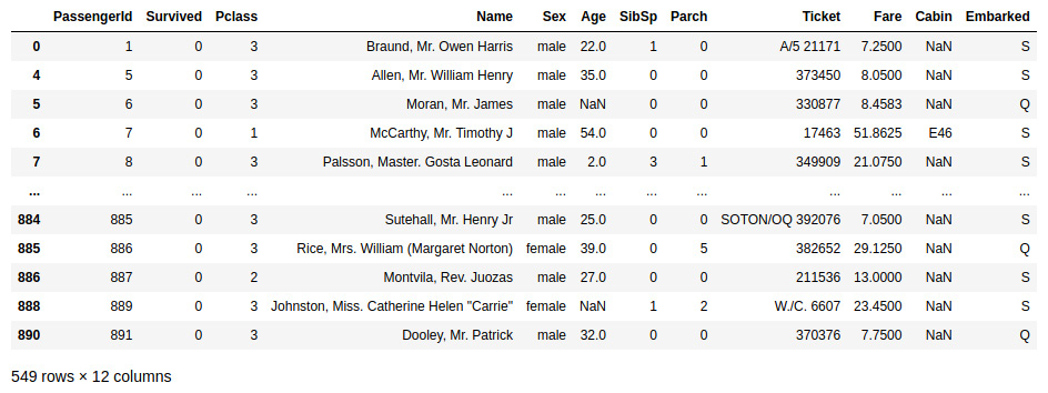
Figure 12.4: Count of the passengers that survived
- After loading the training dataset, load the testing dataset with the following command:
# load the testing dataset
test = pd.read_csv(‘../../Datasets/Titanic/test.csv’)
- Check the result with the test.info() command, which will produce the following result:
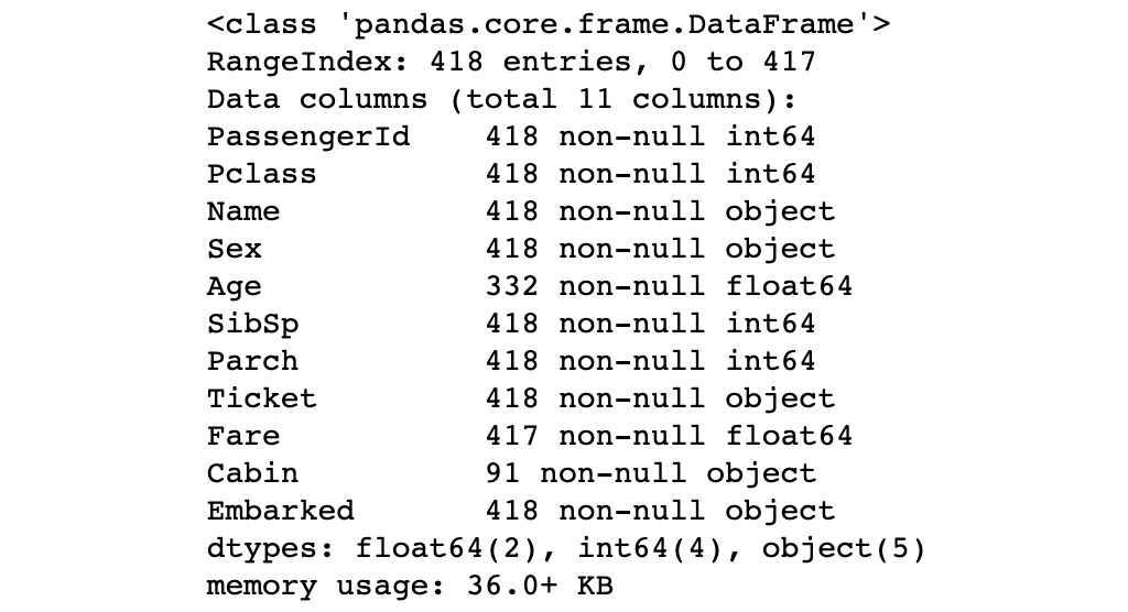
Figure 12.5: Information about the testing dataset
The output shows that there are 418 records in our testing dataset, with the same columns as in the training dataset.
- We’ll now continue to prepare and clean the training dataset as mentioned in Chapter 3, Data Preparation. Machine learning models work best with numerical datatypes for all columns, so let’s convert the Sex column to zeros and ones:
# prepare the dataset
train.Sex = train.Sex.map({‘male’:0, ‘female’:1})
We have now transformed the values in the Sex column to either 0 (for male) or 1 (for female).
- Create the training set, X, which doesn’t contain the Survived output column, using the following code:
# use the values in the Survived column as output targets
y = train.Survived.copy()
X = train.drop([‘Survived’], axis=1)
Since the Survived column contains our output value on which we have to train our model (the target values), we have to extract that from the dataset. We create a new dataset for it called y and then remove the column from the training dataset. We call the new training set X.
Now, let’s do some feature engineering. We can be quite certain that a lot of the columns will not hold any predictive value as to whether a person survived. For example, the name of someone and their passenger ID are interchangeable and will not contribute much to the predictive power of the machine learning model.
- Remove a set of columns that are not needed to predict the surviving passengers:
X.drop([‘Name’], axis=1, inplace=True)
X.drop([‘Embarked’], axis=1, inplace=True)
X.drop([‘PassengerId’], axis=1, inplace=True)
X.drop([‘Cabin’], axis=1, inplace=True)
X.drop([‘Ticket’], axis=1, inplace=True)
We have removed the Name, Embarked, PassengerId, Cabin, and Ticket columns. There is one more thing to do: the Age column contains some empty (null) values. These could get in the way when training the model.
- Replace the empty values with the mean age of all the passengers in the dataset:
X.Age.fillna(X.Age.mean(), inplace=True)
- Let’s have a look at the current size and contents of the training dataset:
X.info()
X.head()
This should give the following output:

Figure 12.6: Dataset information after feature engineering
As becomes clear from this output, the training dataset still holds all the 891 rows but there are fewer columns. Moreover, all columns are of a numerical type – either int64 or float64. To make even better models, there is a lot that data scientists can do. For example, it’s a good option to normalize the columns (get them within the same range) and to do more feature engineering, such as natural language processing, on the non-numerical columns in the source dataset.
- Let’s now train the actual model. We’ll create a logistic regression model, which is essentially a mathematical algorithm to separate the survivors from the people who died in the accident:
from sklearn.linear_model import LogisticRegression
model = LogisticRegression()
model.fit(X, y)
The model.fit method takes the training dataset, X, and the target values, y, and will perform its calculations to make the best fit. This will produce a model, as can be seen in the following output:

Figure 12.7: Fitting the model
- To see what the accuracy of the model is, we can run the full set of test data on the model and see in how many cases the algorithm produces a correct outcome using the following code:
# evaluate the model
model.score(X, y)
You’ll get the following output:
0.8002244668911336
Note
The preceding output will vary slightly. For full reproducibility, you can set a random seed.
A score of 0.8 (and something more) means that the model performs accurately in 80% of the cases in the test set.
We can also get some more understanding of how the model works. Enter the following command:
train.corr()
The resulting correlation graph indicates columns that are closely related:

Figure 12.8: Correlation between columns
A correlation value of 0 indicates no relationship. The further away from 0, a value is, toward a minimum of -1 and a maximum of 1, the stronger the relationship between the columns is. In the table, you can see that the data in the columns Fare and Pclass (the class of the customer) is related since the correlation between them is -0.549500. On the contrary, the columns Age and PassengerId are not related to each other, as expected; since the passenger ID is just an arbitrary number, it would be strange if that was dependent on the age of a person. The column that is most indicative of the survival of a person is Sex; the value of 0.543351 indicates that once you know whether a person is male or female, you can predict whether they survived the disaster with reasonable accuracy. Therefore, the Sex column is a good feature for the model.
- Finally, we have to serialize (export) the model to a file with the pickle framework:
file = open(‘model.pkl’, ‘wb’)
pickle.dump(model, file)
file.close()
The pickle.dump method serializes the model to a model.pkl file in the exercise directory. The file has been opened as wb, which means that it will write bytes to disk. You can check the file exists in the Exercise12.01 folder.
The second part of this exercise is to load the model from disk in an API and expose the API.
- Create a new Python 3 notebook in the Exercise12.01 directory and give it the name production.
Note
The production.ipynb file can be found here: https://packt.live/2ZtjzH7
- In the first cell, enter the following line to install Flask:
!pip install flask
You’ll get the following output:

Figure 12.9: Installing Flask
If Flask is already installed, you will get the following output:

Figure 12.10: Flask already installed
- Now import the required libraries to deserialize the model and to create an API:
from flask import Flask, jsonify, request
import pickle
- The model that we trained in the first part was stored in the model.pkl file. Let’s get that file from disk and deserialize the model into memory:
file = open(‘model.pkl’, ‘rb’) # read bytes
model = pickle.load(file)
file.close()
We now have the same model running in our production environment (the production Jupyter notebook) as in our model training environment (the development notebook from part 1 of this exercise). To test the model, we can make a few predictions.
- Call the predict function of the model and give it an array of values that represent a person; the values are in the same order as the columns of the training set (namely, class, sex, age, number of siblings aboard, number of parents aboard, and fare that was paid) as shown in the following code:
print(model.predict([[3,0,22.0,1,0,7.2500]]))
print(model.predict([[3,1,22.0,1,0,7.2500]]))
You should get the following output:
[0]
[1]
The values in the output (0 and 1) are the predictions of the Survived output field. This means that the model predicted that our first test subject, a man in class 3 of age 22 with 1 child and 0 parents on board who paid 7.25 for the ticket, was more likely to have survived than a woman with the same characteristics.
We have now created a machine learning model that predicts whether a passenger on the Titanic survived the disaster of 1912. But, this model can only be executed by calling it within a Python script.
- Let’s continue with productionizing our model. We first must set up a Flask app, which we’ll call Titanic:
app = Flask(‘Titanic’)
- The app is now an empty API with no HTTP endpoint exposed. To make things a bit more interesting and test whether it works, add a GET method that returns a simple string:
@app.route(‘/hi’, methods=[‘GET’])
def bar():
result = ‘hello!’
return result
After running this cell, test the app by entering and running the following line in a new cell:
app.run()
This will result in an ever-running cell (like an infinite loop), indicated by an
asterisk (*), as shown in the following output:
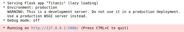
Figure 12.11: Testing the app
The bottom of the cell already indicates what to do: let’s open a new browser window and go to http://127.0.0.1:5000/hi. Since the action that your browser takes is a GET request to the API, you’ll get the correct response back, as you can see in the following figure:

Figure 12.12: Running the app as seen in the browser window
The API now only returns hello! to demonstrate that it’s working technically. We can now continue to add business logic that produces useful results.
- We have to add a new method to the API that executes the model and returns the result as shown in the following code:
@app.route(‘/survived’, methods=[‘POST’])
def survived():
payload = request.get_json()
person = [payload[‘Pclass’],
payload[‘Sex’], payload[‘Age’],
payload[‘SibSb’], payload[‘Parch’],
payload[‘Fare’]]
result = model.predict([person])
print(f’{person} -> {str(result)}’)
return f’I predict that person {person} has
{“_not_ “ if result == [0] else “”}
survived the Titanic ’
These lines define an HTTP POST method under the URL ‘/survived’. When called, a person object is generated from the JSON payload. The person object, which is an array of input parameters for the model, is then passed to the model in the predict statement that we’ve seen before. The result is finally wrapped up in a string and returned to the caller.
Run the app again (stop it by clicking on the interrupt icon (
 ) or by typing Ctrl + C first, if needed). This time, we will test the API with a curl statement. cURL is a program that allows you to make an HTTP request across a network in a similar way to how a web browser makes requests, only the result will be just text instead of a graphical interface.
 - Start a Terminal window (or Anaconda prompt) and enter the following command:
curl -X POST -H “Content-Type: application/json” -d ‘{“Pclass”: 3, “Sex”: 0, “Age”: 72, “SibSb”: 2, “Parch”: 0, “Fare”: 8.35}’ http://127.0.0.1:5000/survived
Note
There is a Jupyter notebook called validation in GitHub that contains the same command in a cell. It can be found here:
The string after the -d parameter in the curl script contains a JSON object with passenger data. The fields for a person have to be named explicitly.
After running this, you’ll see the result of your API call that executed the model as follows in your Terminal or Anaconda prompt:
I predict that person [3, 0, 72, 2, 0, 8.35] has
not survived the Titanic
This output shows that our API works and that the model is evaluated! The API takes the input of one person (the JSON object in the curl statement) and provides it as input to the machine learning model that it has loaded from disk, by deserializing the pickle model.pkl file. The output is wrapped in a string and transferred back to the Terminal across the network.
Note
To access the source code for this specific section, please refer to https://packt.live/306HgE5.
By completing this exercise, you have practiced a lot of useful techniques. You have built and trained a machine learning model, stored your model as a pickle file, and used the file in a deserialized form in an API using the Flask framework. This has resulted in an application that can predict whether a passenger of the Titanic survived the disaster of 1912 or not. The API can be used from any other application that can access it across a network. In the following activity, you’ll perform the same steps to build an API that predicts in which class a passenger was sitting.
Activity 12.01: Predicting the Class of a Passenger on the Titanic
In this activity, you’ll use the same dataset as in the previous exercise. Rather than building a model that predicts whether a person survived the Titanic disaster, we’re going to try to predict which class (1, 2, or 3) a person was in based on their details.
Note
The code for this activity can be found here:
Perform the following steps to complete the activity:
- Start Jupyter Notebook and create a new Python 3 notebook in the same directory, with the name development.
- Install the pandas and sklearn Python libraries for model building and import them into your notebook.
- Load the training data into a Pandas DataFrame object called train.
- Convert the Sex column to zeros and ones.
- Create a new dataset for the output values (in the Pclass column). Call that dataset y and then remove the Pclass column from the training dataset. Call the new training set X.
- Remove the columns that you cannot parse or that don’t contain good features for your model.
- Replace the empty values in the Age column with the fillna method.
- Create a logistic regression model with the sklearn.linearmodel.LogisticRegression class.
- Serialize the model to a file with the pickle.dump method. Check that the model file exists in the Activity12.01 folder.
- Create a new Python 3 notebook in the Activity12.01 directory and give it a meaningful name such as production.
- In the new notebook, install Flask and import the required libraries to deserialize the model and to create an API.
- Load the model file from disk and deserialize the model into memory.
- Set up a Flask app called ClassPredictor.
- Define an HTTP POST method under the URL ‘/class’, by making use of the Flask method annotation @app.route(‘/class’, methods=[‘POST’]). When called, a person object (an array of input parameters) should be generated from the JSON payload. The result of the model should be wrapped up in a string and returned to the caller.
- Run the app with an app.run() statement and test the API with a curl statement. You should get an output similar to the following:
I predict that person [1, 0, 72, 2, 0,28.35] was
in class [2] of the Titanic
You have now completed an activity to train a model and build an API for it. In the next part of this chapter, we are going to explore options to productionize these kinds of services in a live application.
Note
The solution to this activity can be found on page 654.
Deploying Models to Production
After creating an API that contains your machine learning model, it has to be hosted in a production environment. There are several ways to do this, such as the following, for example:
- By copying the API to a (virtual) server
- By containerizing the API and deploying the container to a cluster
- By installing the API in a serverless framework such as Amazon AWS Lambda or Microsoft Azure Functions
We’ll focus on the practice that is very common nowadays and still gaining popularity: containerizing the API and model.
Docker
AI applications usually work with large datasets. With “big data” comes the requirement for scalability. This means that models in production should scale in line with the data. One way to scale your software services is to distribute them in containers. A container is a small unit of computational power, similar to a virtual machine. There are many other advantages when containerizing your software: deployment becomes easier and more predictable since the containers stay the same in every environment.
The best framework for containerizing applications is Docker. This open-source tool has become the de facto way to containerize applications. Docker works with the concepts of images and containers. An image is a template of an application that is deployable to an environment. A container is a concrete implementation of an image. What’s inside an image (and in its resulting containers) is very flexible; it can range from a simple “hello world” script to a full-blown enterprise application. It’s considered good practice to build Docker images for a single purpose and have them communicate with each other via standard protocols such as REST. In this way, it’s possible to create infrastructure and software by carefully selecting a set of Docker images and connecting them. For example, one Docker image might contain a database and the data of an application itself. Another Docker image can be created to hold the business logic and expose an API. A third Docker image could then contain a website that is published on the internet. In the next part, about Kubernetes, you will see an example diagram of such an application architecture. In our other exercise and activity in this chapter, we’ll use Docker to productionize a machine learning model.
Docker in itself is not so useful in an enterprise; an environment is needed where Docker images can be published and maintained. One of the most popular frameworks to do so is Kubernetes, which we’ll discuss next.
Kubernetes
To create a cluster of many containers, and thus to generate scale in an application, a tool needs to be used that can manage those containers in one environment. Ideally, you would want to deploy many containers with the same software and treat them as if they were one unit. This is exactly the purpose of frameworks such as Kubernetes, Docker Swarm, and OpenShift. They allow software developers to distribute their applications across many “workers,” which are, for example, cloud-based nodes. Kubernetes was created by Google to be used in their cloud computing cluster. It was made open source in 2015. Nowadays, it’s one of the most popular frameworks for scaling software applications. The large Kubernetes community is very active.
Kubernetes works with the concepts of Pods and Nodes. A Pod is the main abstraction for an application; you always deploy an application in one or more Pods. A Kubernetes cluster consists of Nodes, which are the worker servers that run applications. There is always one Master Node that is responsible for managing the cluster. The following figure gives an overview of this model:

Figure 12.13: Kubernetes cluster (redrawn from https://kubernetes.io/docs/)
In the previous figure, you see a Kubernetes cluster with four nodes. One of the nodes has the Master role and contains one Deployment. From the Deployment, an application can be deployed onto the other Nodes. Once an application is deployed to nodes in a Kubernetes cluster, it runs in a Pod. A Pod contains a group of resources such as storage and networking that are needed to run a container. In the previous figure, there are three nodes. On one of them, there is a Pod that contains an application (the containerized app). If we zoom in on a Node, we can see a structure such as in the following figure:

Figure 12.14: Kubernetes Node with Pods (redrawn from https://kubernetes.io/docs/)
In the preceding figure, you can see one Node with four Pods in it. Each Pod has its function and contents; for example, the Pod with ID 10.10.10.4 contains three containerized apps and two storage volumes, which work together toward a business goal such as providing a website. You can see that each Node has two core processes running: kubelet for communication, and Docker for running the images. The Kubernetes command-line interface is called kubectl.
Note
If you want to read more about Kubernetes and Docker, please refer to the following link for the official documentation: https://kubernetes.io/docs/home/
In the next exercise, you will learn how to dockerize an API that contains a machine learning model, and how to deploy it to a Kubernetes cluster.
Exercise 12.02: Deploying a Dockerized Machine Learning API to a Kubernetes Cluster
In this exercise, we’ll store a machine learning API as a Docker image, and deploy an instance (a container) to a Kubernetes cluster. This exercise is a follow-up of the previous exercise, so make sure you have completed that one.
In Exercise 12.01, Creating a Machine Learning Model API with pickle and Flask That Predicts Survivors of the Titanic, you created a machine learning model that predicts whether a person survived the Titanic disaster in 1912. You created an API that contains the model. We will be using that model in this exercise. The final goal of this exercise is to deploy the same model to a Kubernetes cluster.
We will not work with Jupyter in this exercise; we’ll do most of the work from Command Prompt and a text editor (or IDE).
Before you begin, follow the installation instructions in the Preface to install Docker and Kubernetes.
This exercise consists of two parts. In the first part, we’ll create a Docker image and publish it to a local registry. In the second part, we’ll run the image in a Kubernetes cluster.
Perform the following steps to complete the exercise:
- Create a new directory, Exercise12.02, in the Chapter12 directory to store the files for this exercise.
- Copy the model.pkl file from the Chapter12/Exercise12.01 directory into the Exercise12.02 directory.
- Let’s create a new API first. Since we’ll work outside of Jupyter on this one, we have to make sure that it runs on our local machine. Create a new file in the Exercise12.02 folder called api.py. Open it with a text editor or an IDE and enter the following Python code:
from flask import Flask, request
import pickle
# load the model from pickle file
file = open(‘model.pkl’, ‘rb’) # read bytes
model = pickle.load(file)
file.close()
# create an API with Flask
app = Flask(‘Titanic’)
# call this: curl -X POST -H “Content-Type: application/json”
# -d ‘{“Pclass”: 3, “Sex”: 0, “Age”: 72, “SibSb”: 2, “Parch”: 0,
#”Fare”: 8.35}’ http://127.0.0.1:5000/survived
@app.route(‘/survived’, methods=[‘POST’])
def survived():
payload = request.get_json()
person = [payload[‘Pclass’], payload[‘Sex’],
payload[‘Age’], payload[‘SibSb’],
payload[‘Parch’], payload[‘Fare’]]
result = model.predict([person])
return f’I predict that person {person} has
{“_not_ “ if result == [0] else “”}survived the Titanic ’
app.run()
This code is the same as in the production notebook of Exercise 12.01, Creating a Machine Learning Model API with pickle and Flask That Predicts Survivors of the Titanic, but is now pulled together in one executable Python file since it’s the most efficient way to run a Python program. It uses the machine learning model in the pickle model.pkl file to predict whether a person survived the Titanic disaster.
- Open a new Terminal or Anaconda Prompt and navigate to the Exercise12.02 folder using the cd command. Enter the following command to check whether the API is working:
python api.py
If all is OK, you should get the message that your API is running on localhost, as seen in the following screenshot:

Figure 12.15: Running the API
- Test the local API by opening a new Terminal or Anaconda Prompt and enter the following code:
curl -X POST -H “Content-Type: application/json” -d ‘{“Pclass”: 3, “Sex”: 0, “Age”: 72, “SibSb”: 2, “Parch”: 0, “Fare”: 8.35}’ http://127.0.0.1:5000/survived
You’ll get the following output in the same Terminal, indicating that the API is working and that we get good predictions from the model:
I predict that person [3, 0, 72, 2, 0, 8.35] has
not survived the Titanic
- Add a new file in the Exercise12.02 folder with the name requirements.txt. If we will deploy the API to another environment, it’s good practice to indicate which libraries were used. To do so, Python offers the requirements.txt file, where you can write the dependencies of an application.
- Open the requirements.txt file in an editor and enter the following lines:
Flask
sklearn
pandas
This simple line is enough for our API. It indicates that we are depending on the Flask, sklearn, and pandas libraries for everything to work. Since pickle is a standard Python library, we don’t have to reference it explicitly. The requirements file is used in the Docker image once it runs in production.
Note
It’s possible to specify the exact version, for example, by entering Flask==1.1.1. To see which version you have in your development environment, enter pip freeze. To export the current list of dependencies and store them as requirements.txt, enter pip freeze > requirements.txt.
Now, let’s continue with containerizing the API to make it ready to deploy to a production environment. We need to create a Docker image, which is a template for creating the actual Docker containers that will be deployed.
- First, let’s verify that Docker is installed correctly on your system. If you have followed the installation instructions, enter the following command in a new Terminal or Anaconda Prompt:
sudo docker run hello-world
This command will get a basic Docker image called hello-world from the central repository (Docker Hub). Based on that image, a local container will be created on your local machine. The output will be as follows:

Figure 12.16: Output of running the ‘hello-world’ Docker image
- You can check the images you have stored on your local machine by typing the following:
sudo docker image ls
This will give an output like the following:

Figure 12.17: Checking stored images
At the moment, we only see the hello-world image that was created in the previous step.
- Instead of working with a pre-defined Docker image, we want to set up our own Docker images that are defined in strict files that are named Dockerfile. So, let’s add a new text file in the same directory and call it Dockerfile (without an extension). Open Dockerfile in a text editor or IDE, enter the following code, and save the file:
FROM python:3.7
RUN mkdir /api
WORKDIR /api
ADD . /api/
RUN pip install -r ./requirements.txt
EXPOSE 5000
ENV PYTHONPATH=”$PYTHONPATH:/api”
CMD [“python”, “/api/api.py”]
Dockerfile is the most important artifact when creating your images. There are five main parts to our file.
First (line 1), a base image is acquired. In our case, this is a Python 3.7 image that can run Python applications.
Next (lines 3 to 5), the contents of the current directory are added to the image; this ensures that the api.py and requirements.txt files are packaged within the container. We add all files to a directory called api.
Next (line 7), the required Python libraries that we marked as dependencies in the requirements.txt file are installed with the pip install command. In our case, this is just the Flask library.
Next (line 8), we tell Docker to expose network port 5000 to the outside world. If this is omitted, the API cannot be reached from the network.
Finally (lines 11 and 12), we start the API by setting the Python path to the api directory and executing the python api/api.py command. This is the same command that we tested locally in Step 3 of this exercise.
- Open a new Terminal window (or Anaconda Prompt) in the Exercise12.02 directory and enter the following command to create an image:
sudo docker build -t titanic .
This command will pull the base image (with Python 3.7) from Docker Hub and then follow the other instructions in the default Dockerfile (called Dockerfile). The . at the end of the command points to the current directory. The -t parameter specifies the name of our image, titanic. The command might take some time to complete. Once the script completes, this is the expected output:
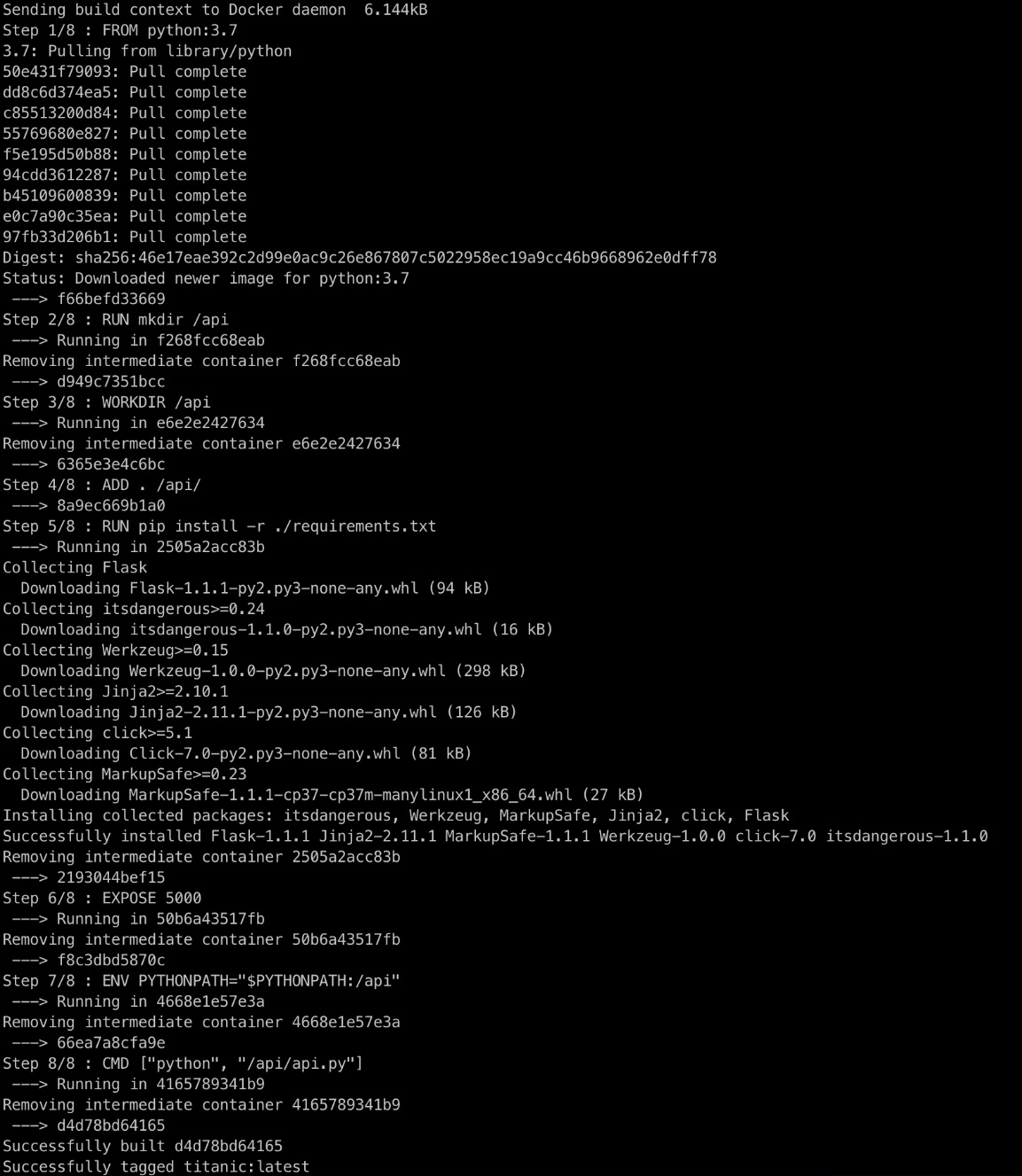
Figure 12.18: Building a Docker image
In the output, it becomes clear that all steps in our Dockerfile have been followed. The Flask library is loaded, port 5000 is exposed, and the API is running.
- Let’s check our local image repository again:
sudo docker image ls
Next to the hello-world image, you’ll see the base Python 3.7 image and our Titanic API:

Figure 12.19: Checking stored images
It’s great that we have a Docker image now, but that image has to be published to a Docker registry when we want to deploy it. Docker Hub is the central repository, but we don’t want our Titanic API to end up there.
- Create a local registry and publish our image there, ready to be deployed to Kubernetes in the next part of this exercise. Enter the following command in your Terminal:
docker run -d -p 6000:5000 --restart=always --name registry registry:2
This will download the registry libraries and will run a local registry. The output is as follows:
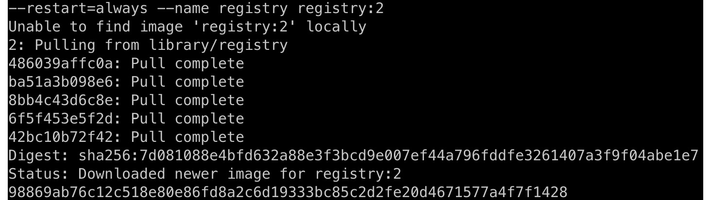
Figure 12.20: Creating a local registry
- Tag your Docker image with the following command, to give it a suitable name:
docker tag titanic localhost:6000/titanic
- Now, push the titanic image to the running local registry with the following command:
docker push localhost:6000/titanic
This generates the following output:

Figure 12.21: Pushing a Docker image to a local registry
- To verify that your image is pushed to the local registry, enter the following command:
curl -X GET http://localhost:6000/v2/titanic/tags/list
If all is well, you’ll see the image with the latest tag:
{“name”:”titanic”,”tags”:[“latest”]}
- Double-check that all is OK by entering the docker image ls and docker ps commands. You’ll have a similar output:
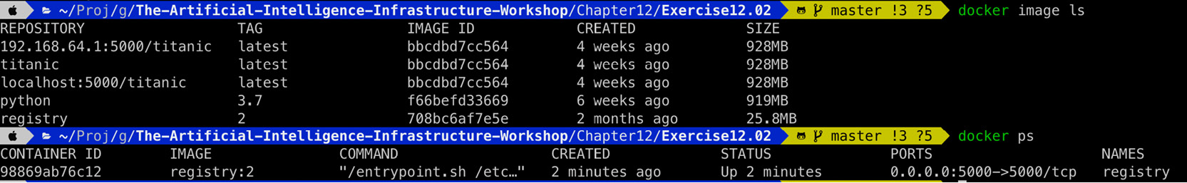
Figure 12.22: Viewing the Docker images and containers
As you can see in the output, the titanic image is now also available as localhost:6000/titanic. The registry image is new, and it has a running container called registry:2. We have just successfully published our titanic image to that registry.
In the second part of this exercise, we’ll use the Docker image to host a container on a Kubernetes cluster.
- We first have to make sure that Minikube, the local version of Kubernetes, is running. Minikube is, in fact, a local virtual machine. Type the following command in a new Terminal or Anaconda Prompt:
minikube version
If all is OK, this will produce an output like minikube version: v1.8.1, along with a commit hashtag, as follows:
minikube version: v1.8.1
commit: cbda04cf6bbe65e987ae52bb393c10099ab62014
- Start minikube by entering the following command in a new Terminal window or Anaconda Prompt:
minikube start --insecure-registry=”localhost:6000”
If you’re running within a virtual machine like VirtualBox, the command will be minikube start --driver=none. If all goes well, you’ll get the following output:
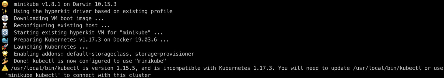
Figure 12.23: Starting Minikube
- Confirm that Minikube is running by using the following command:
minikube status
You’ll get a status update like the following:
host: Running
kubelet: Running
apiserver: Running
kubeconfig: Configured
If you want to look even further into your Kubernetes cluster, start up a dashboard with the following command:
minikube dashboard
This will open a browser window with a lot of useful information and configuration options:
Figure 12.24: The Kubernetes dashboard
- We have to connect our now-running Minikube Kubernetes cluster to a command-line interface, called kubectl. Type in the following command in your Terminal or Anaconda Prompt, as was already suggested in the previous output:
minikube kubectl
This will produce an output like the following:

Figure 12.25: Connecting Minikube to your kubectl command
You can read the kubectl controls the Kubernetes cluster manager line, which indicates that we can now use the kubectl tool to give commands to our cluster. You can get more information about the cluster with the kubectl version and kubectl get nodes commands:
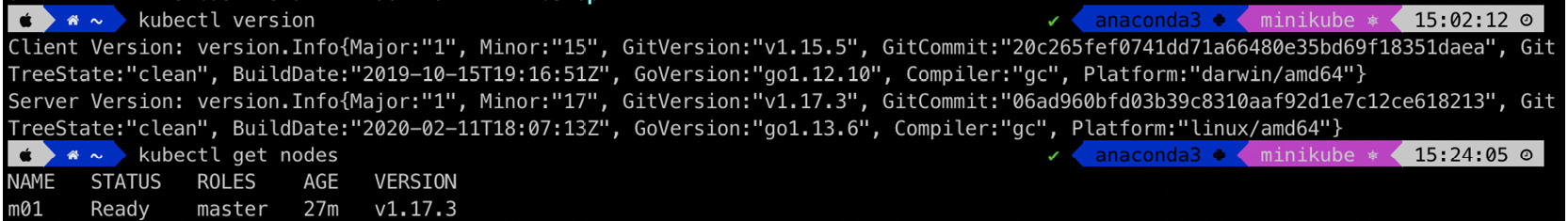
Figure 12.26: Getting information from Minikube
- We have already created a Docker image and practiced deploying that to a Docker registry in part 1 of this exercise. We’ll rebuild the image now, but with the Docker daemon (process) of the Kubernetes cluster to make sure it lands on the Minikube cluster. Start by entering the following command:
eval $(minikube docker-env)
This command points our Terminal to use a different docker command, namely, the one in the Minikube environment.
- Let’s build the container again but now with Minikube. Enter the following command:
docker build -t titanic .
You’ll get the same output as in part 1 of this exercise.
- Now all that’s left to do is to deploy our Docker image to the cluster and run it as a container. For this, we create a Kubernetes deployment with the following command:
kubectl run titanic --image=titanic --image-pull-policy=Never
If this is successful, you’ll see the following output:
deployment.apps/titanic created
- Verify the deployment of the container with the following command:
kubectl get deployments
This will produce a list of deployed containers:

Figure 12.27: Retrieving a list of deployed containers from Kubernetes
You can also check the Kubernetes dashboard if you have started it, and check whether the deployment and Pod have been created:
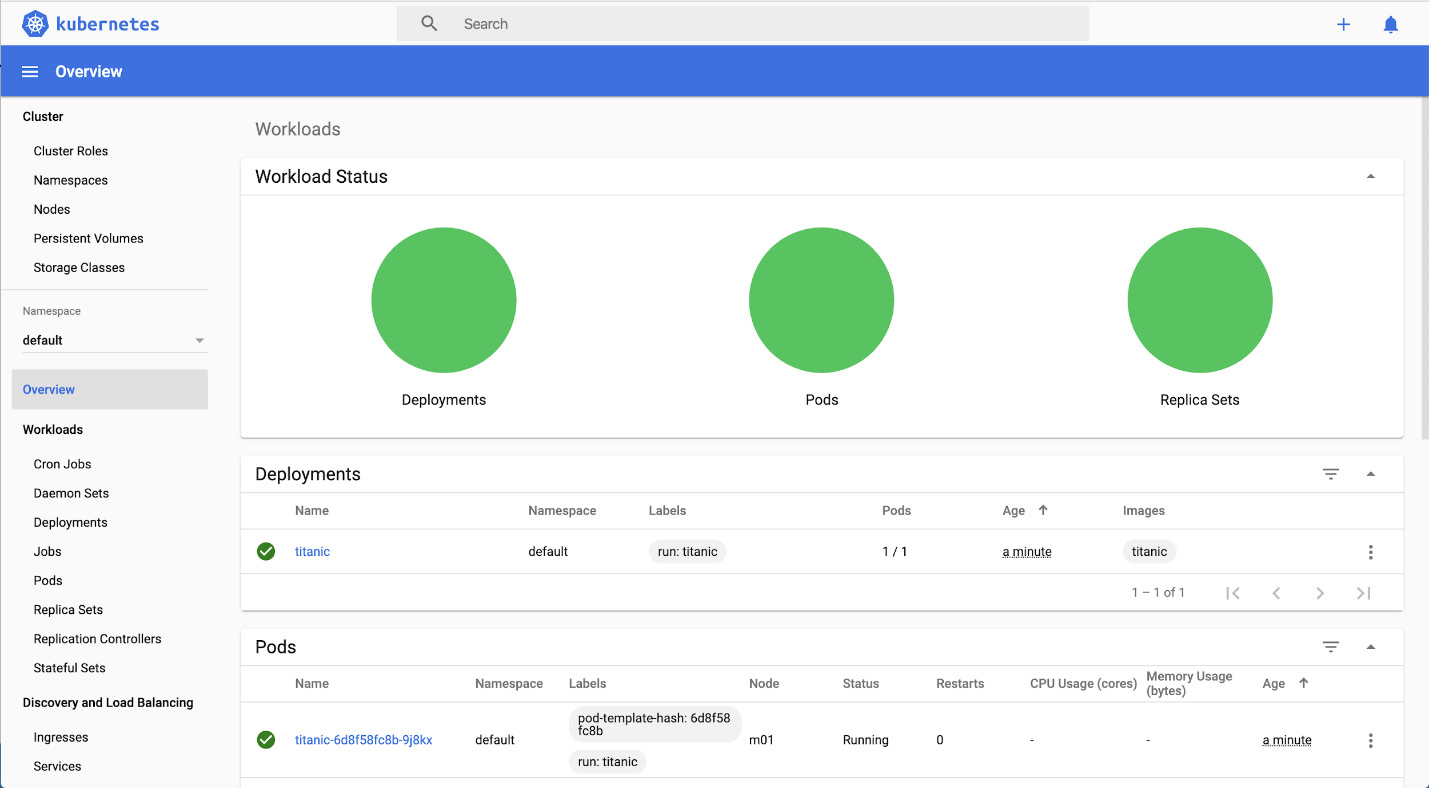
Figure 12.28: The Kubernetes dashboard
- Now that our app is deployed, we want to connect to the Titanic API. By default, the running containers can only be accessed by other resources (containers) in the same Kubernetes Pod. There are several ways to connect to our app from the outside world, such as an Ingress and Load Balancer. To keep it simple, we will just instruct our cluster to forward the network traffic on port 5000 to our running Pod in the Minikube cluster:
kubectl port-forward titanic-6d8f58fc8b-znmx9 5000:5000
Note
In the preceding code, replace the name of the pod with your own; you can find it in the Kubernetes dashboard or by entering kubectl get pods
This will create a local task that forwards network traffic to the titanic Pod. You will have the following output:
Forwarding from 127.0.0.1:5000 -> 5000
Forwarding from [::1]:5000 -> 5000
- To test the API, enter the following command in a new terminal window (while keeping the port forwarding running):
curl -X POST -H “Content-Type: application/json” -d ‘{“Pclass”: 2, “Sex”: 1, “Age”: 34, “SibSb”: 1, “Parch”: 1, “Fare”: 5.99}’ http://127.0.0.1:5000/survived
This sends a JSON string through the proxy to the running container in our Minikube Kubernetes cluster. If all goes well, you’ll get the output of a prediction in the familiar form, in the same Terminal where you executed the curl command:
I predict that person [2, 1, 34, 1, 1, 5.99] has
survived the Titanic
Note
To access the source code for this specific section, please refer to https://packt.live/32s2PC3.
By completing this exercise, you have containerized a machine learning API and have published it to a Docker registry. You have also gained experience with deploying Docker images to a Kubernetes cluster. Together, this gives you the skills to publish a machine learning model in production.
In the next activity, you’ll deploy a machine learning model to a Kubernetes cluster that predicts the class of a Titanic passenger.
Activity 12.02: Deploying a Machine Learning Model to a Kubernetes Cluster to Predict the Class of Titanic Passengers
In this activity, you will deploy the machine learning model that you created in Activity 12.01, Predicting the Class of a Passenger on the Titanic, to predict the passenger class of a person on board the Titanic to a Kubernetes cluster.
Note
The code for this activity can be found here:
Perform the following steps to complete the activity:
- To start, copy the model.pkl file from the Chapter12/Activity12.01 directory into a new Activity12.02 directory.
- Create a new file in the Activity12.02 folder called api.py.
- Open a new Terminal or Anaconda Prompt and navigate to the Activity12.02 folder. Enter the following command to check whether the API is working:
python api.py
If all is OK, you should get the message that your API is running on localhost.
- Test the local API by opening a new Terminal or Anaconda Prompt and enter the following command:
curl -X POST -H “Content-Type: application/json” -d ‘{“Survived”: 0, “Sex”: 1, “Age”: 52, “SibSb”: 1, “Parch”: 0, “Fare”: 82.35}’ http://127.0.0.1:5000/class
- Add a new requirements.txt file, open it in an editor, and enter the lines to import the Flask, sklearn, and pandas libraries.
- Add a new file in the same directory and call it Dockerfile.
- Enter the docker build command to create an image with the right tag. In the output, it should become clear that all steps in our Dockerfile have been followed. The Flask library is loaded, port 5000 is exposed, and the API is running.
- Create a local Docker registry and publish the titanic image.
- Tag your Docker image.
- Push the titanic image to the running local registry.
- To verify that your image is pushed to the local registry, enter the following command:
curl -X GET http://localhost:6000/v2/titanic/tags/list
- Start and confirm minikube in a new Terminal window or Anaconda Prompt.
- Startup a minikube dashboard.
- Point your Terminal to the docker command of the Minikube cluster.
- Build the container again but now with the Minikube daemon.
- Create a Kubernetes deployment. If this is successful, you’ll see the deployment.apps/titanic created statement.
- Verify the deployment of the container by checking the Kubernetes dashboard.
- Create a network connection that allows communication (via port forwarding) between the outside world and the resources in your Pod on the Minikube cluster.
- Test the API using the following command:
curl -X POST -H “Content-Type: application/json”
# -d ‘{“Survived”: 1, “Sex”: 0, “Age”: 72, “SibSb”: 2, “Parch”: 0, “Fare”: 68.35}’ http://127.0.0.1:5000/class
This will produce the following output:
I predict that person [1, 0, 72, 2, 0, 68.35] was
in passenger class [1] of the Titanic
You have now successfully dockerized an API with a machine learning model, and deployed the Docker image to a Kubernetes cluster. In the real world, this is a common approach to productionize software in a cloud environment.
Note
The solution to this activity can be found on page 661.
In the next section, we’ll explore how to deploy machine learning models to an ever-running streaming application.
Model Execution in Streaming Data Applications
In the first part of this chapter, you learned how to export models to the pickle format, to be used in an API. That is a good way to productionize models since the resulting microservices architecture is flexible and robust. However, calling an API across a network might not be the best-performing way to get a forecast. As we learned in Chapter 2, Artificial Intelligence Storage Requirements, latency is always an issue when working with high loads of event data. If you’re processing thousands of events per second and have to execute a machine learning model for each event, your network and pickle file that’s stored on disk might not be able to handle the load. So, in a similar way to how we cache data, we should cache models in memory as close to the data stream as possible. That way, we can reduce or even eliminate the network traffic and disk I/O. This technique is often used in high-velocity stream processing applications, for example, fraud detection in banks and real-time recommendation systems for websites.
There are several methods of caching models in memory. Some platforms offer built-in capabilities. For example, the H2O.ai platform has the option to export models to a POJO/MOJO binary object. Spark has its machine learning library called SparkML, which is quite extensive and easy to use. All these methods have one disadvantage: they require a lock-in with the platform. It’s not possible to distribute a model from H2O.ai to DataBricks, or from Spark to DataIku. To enable this kind of flexibility, an intermediate format has to be picked as the “glue” between data scientists and data engineers that gives both practitioners the freedom to choose the tools they want. PMML is such a format, and we’ll discuss it in the next section.
PMML
As this book is focused on open source standards, we have picked a popular intermediate model format that we can load in memory – PMML, short for Predictive Model Markup Language. A PMML file is an XML-based file that contains the input parameters, calculations of the algorithms, and output field of a model. Exporting a model to PMML is essentially a way of serializing a model, similar to how exporting to pickle works. A PMML file can be read quite easily by humans, as can be seen in the following figure:

Figure 12.29: Example of a PMML file with a simple logistic regression model
The PMML format is maintained by the Data Mining Group, which is an independent, non-profit consortium of organizations. There is also a JSON-based format for models called Portable Format for Analytics (PFA). Since that format is still emerging and thus less mature than PMML, we will not discuss it further in this book. The next paragraph contains a short introduction to a popular stream processing framework, Apache Flink.
Apache Flink
Apache Flink is one of the most popular streaming engines, and for a good reason. It offers low latency and high throughput for streaming data processing and gives a lot of power to developers. Compared to Spark Structured Streaming, another popular stream processing framework, it offers more features and better performance. A Flink job is a Java application that can be executed on a local machine or within a cluster.
In the next exercise, you’ll practice with PMML and Flink by creating a real-time stream processing application that includes a machine learning model.
Exercise 12.03: Exporting a Model to PMML and Loading it in the Flink Stream Processing Engine for Real-time Execution
In this exercise, you’ll create a simple machine learning model, export it to PMML, and load it in memory to be used in a data stream.
Before you begin, follow the installation instructions in the Preface to install Java, Maven, Netcat, and a suitable IDE (IntelliJ IDEA or Eclipse).
Perform the following steps to complete the exercise:
- In the Chapter12 directory, create the Exercise12.03 directory to store the files for this exercise.
- Open Jupyter Notebook and create a new Python 3 notebook called export_pmml in the Exercise12.03 folder.
- Copy the model.pkl file from the Exercise 12.01 directory to the Exercise12.03 directory. This can be done manually, or with the following statement in a notebook:
!cp ../Exercise12.01/model.pkl .
- Enter the following line in the first cell of the new notebook:
!pip install sklearn2pmml
This will install the required library, which can export our models to the PMML format:

Figure 12.30: Installation of sklearn2pmml
If sklearn2pmml is already installed, you will have the following output:
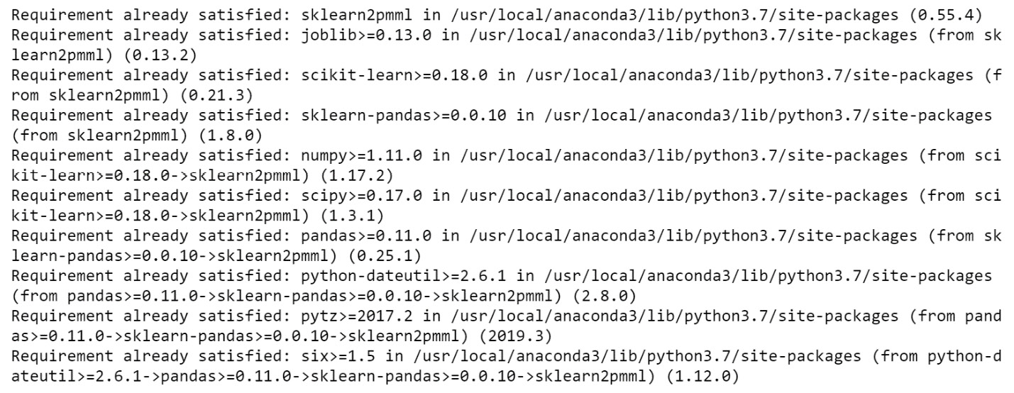
Figure 12.31: sklearn2pmml already installed
- Create a new cell and enter the following lines to start using the pickle and sklearn2pmml libraries:
from sklearn2pmml import sklearn2pmml, make_pmml_pipeline
import pickle
- Deserialize the pickled model by executing the following code in a new cell:
file = open(‘model.pkl’, ‘rb’) # read bytes
model = pickle.load(file)
file.close()
Now we can export the model to the PMML format.
- Enter the following lines in a new cell to create a pipeline, export the method, and write it to the PMML file:
pmml_pipeline = make_pmml_pipeline(model)
sklearn2pmml(pmml_pipeline, ‘titanic.pmml’)
First, we create a pipeline model, which is another representation of the model. Then, we call the sklearn2pmml method that performs the export and writes the resulting PMML file (titanic.pmml) to disk.
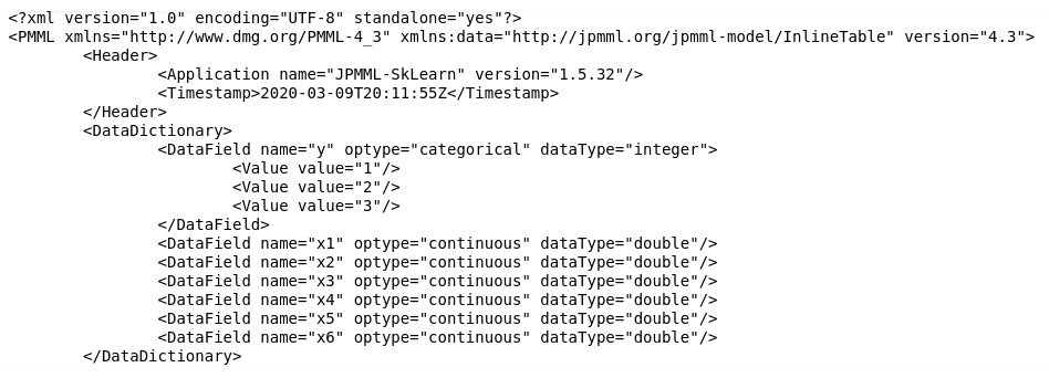
- Check the contents of the generated titanic.pmml file by entering the following line in a new cell:
!cat titanic.pmml
This will produce the following output:

Figure 12.32: Viewing the contents of a PMML model
As you can see, the PMML file is an XML-structured file that is quite easy to read. The input and output fields are listed, and the type of model becomes clear from the <RegressionModel> tag.
Now let’s create a streaming job. We’ll use Apache Flink for this. We’ll write the code with an example from IntelliJ IDEA. You can also choose another IDE. It’s also possible (though not recommended) to use a plain text editor and run the code from a Terminal or command line.
- Open a new Terminal window in the Exercise12.03 directory and enter the following lines to set up Apache Flink:
mvn archetype:generate
-DarchetypeGroupId=org.apache.flink
-DarchetypeArtifactId=flink-quickstart-java
-DarchetypeVersion=1.10.0
- During the installation, enter the following values:
groupId: com
artifactId: titanic
version: 0.0.1
package: packt
This will generate a project from a template.
- Open your favorite IDE (IntelliJ IDEA, Eclipse, or another) and import the generated files by selecting the pom.xml file (if you use Eclipse, the m2e plugin allows you to import Maven projects) as shown in the following figure:
Figure 12.33: Importing a Maven project into IntelliJ IDEA
- The Flink project that was generated by running the mvn archetype:generate command contains two Flink jobs: one for streaming data, and one for batch processing. Since we don’t need the one for batch processing in this exercise, remove the src/main/java/packt/BatchJob.java file. Copy the titanic.pmml file that we created in Step 8 to the titanic/src/resources directory. You’ll see the following file structure:

Figure 12.34: File structure of the generated Flink project
- If you installed JDK and Maven, you should be able to compile the code. Type the following in your Terminal to compile the code and package it into a JAR file:
mvn clean package
This produces the following output:

Figure 12.35: Output of the Maven package command
In the output, you’ll see BUILD SUCCESS, which indicates that you now have a working Java program.
Let’s start by testing the job – first, the Maven template-generated code that can be deployed to a Flink cluster.
- Since we want to test locally first, let’s change the configuration a bit. Open the pom.xml file and remove the <provided> tags in the dependencies of flink-java and flink-streaming-java; these tags are single lines within the <dependency> elements. The file will look like the following:
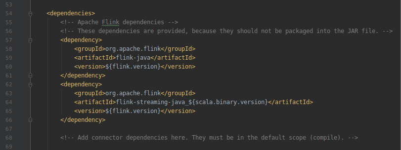
Figure 12.36: The pom.xml file with provided tags removed for Flink dependencies
Save the file, then import the Maven changes.
- Open the StreamingJob.java file in your IDE and add the following lines at the top:
import org.apache.flink.api.common.
serialization.SimpleStringEncoder;
import org.apache.flink.core.fs.Path;
import org.apache.flink.streaming.api.
datastream.DataStream;
import org.apache.flink.api.common.
functions.MapFunction;
import org.apache.flink.streaming.api.datastream.
SingleOutputStreamOperator;
import org.apache.flink.streaming.api.environment.
StreamExecutionEnvironment;
import org.apache.flink.streaming.api.functions.
sink.filesystem.StreamingFileSink;
These lines will add the necessary Flink libraries to our class file.
- In the middle part of the file, within the main function, add the following lines:
DataStream<String> dataStream = env.socketTextStream(
“localhost”, 1234, “ ”);
StreamingFileSink<String> sink = StreamingFileSink
.forRowFormat(new Path(“out”),
new SimpleStringEncoder<String>(“UTF-8”))
.build();
dataStream.addSink(sink);
This code sets up a data stream that listens to a local socket on port 1234. It takes the lines and writes (sinks) the lines to a file in the out directory.
- To write to a local socket, we use the Netcat tool. Test the simple code by opening a Terminal and typing the following command:
nc -l -p 1234
You get a prompt to enter lines. Leave it open for now.
- Type the following in a Terminal to build and run the code:
mvn clean package
mvn exec:java -Dexec.mainClass=”packt.StreamingJob”
These lines are the Maven instructions to compile the code, package it into a JAR file, and run the file with the entry point in the packt.StreamingJob class that contains our main function.
- In the Terminal that’s still running Netcat, type the following lines of text followed by Enter for each line:
hello!
this
is a test
to check
if Flink is writing
data to a file
You should get the following output:

Figure 12.37: Running a Flink job that processes input from a local socket
- Now check the output in the titanic_results directory. You should see a subfolder with a date and time, and a file for each line that was entered in the input socket:

Figure 12.38: Checking the file contents that were produced by the Flink job
- Let’s make our application a bit more interesting by using input for our machine learning model. We have to add some dependencies to our project for this. Add the following lines to pom.xml and import the Maven changes:
<dependency>
<groupId>org.jpmml</groupId>
<artifactId>pmml-evaluator</artifactId>
<version>1.4.15</version>
</dependency>
<dependency>
<groupId>org.jpmml</groupId>
<artifactId>pmml-evaluator-extension</artifactId>
<version>1.4.15</version>
</dependency>
- Edit the StreamingJob.java file again and add the following lines at the top of the file:
import org.dmg.pmml.FieldName;
import org.jpmml.evaluator.*;
import org.jpmml.evaluator.
visitors.DefaultVisitorBattery;
import java.io.File;
import java.util.LinkedHashMap;
import java.util.List;
import java.util.Map;
These lines import the required PMML and common Java libraries for working with PMML files.
- Enter the following lines at the beginning of the main method:
// prepare PMML evaluation
ClassLoader classloader= StreamingJob.class
.getClassLoader();
Evaluator evaluator= new LoadingModelEvaluatorBuilder()
.setLocatable(false)
.setVisitors(new DefaultVisitorBattery())
.load(newFile(classLoader.getResource(
“titanic.pmml”).getFile())).build();
List<? extends InputField> inputFields =
evaluator.getInputFields();
This code deserializes the model from PMML, loading the model in memory ready to be executed. The list of input fields will come in handy in the next step.
We are now ready to parse incoming messages as persons that can be evaluated according to whether they survived the Titanic disaster. The input values will be in a comma-separated string with the values “class, sex, age, number of siblings on board, number of parents on board, and fare paid”. For example, “3,0,28,2,0,9.45” indicates a man of 28 years old who entered the ship with his two children.
- The PMML evaluator expects a map of FieldName value objects, so we first have to convert the input strings. To do so, add the following lines to the class:
SingleOutputStreamOperator<String> mapped =
dataStream.map(new MapFunction<String, String>() {
@Override
public String map(String s) throws Exception {
System.out.println(“EVENT: “ + s);
Map<FieldName, FieldValue> arguments = new LinkedHashMap<>();
String[] values = s.split(“,”);
// prepare model evaluation
for (int i = 0; i < values.length; i++) {
FieldName inputName = inputFields.get(i).getName();
FieldValue inputValue = inputFields.get(i)
.prepare(values[i]);
arguments.put(inputName, inputValue);
}
// execute the model
Map<FieldName, ?> results = evaluator.
evaluate(arguments);
// Decoupling results from the
//JPMML-Evaluator runtime environment
Map<String, ?> resultRecord = EvaluatorUtil.decodeAll(results);
System.out.println(resultRecord);
return s;
}
});
This code adds a map method to the stream processing job that splits the input string and uses the resulting string values to build a set of arguments for the machine learning model.
- Now, if you run this code together with Netcat for the input socket, you can get real-time predictions from the model. Enter the following set of comma-separated values in the nc prompt that is already running, followed by Enter, and see what predictions are made:
3,0,28,2,0,9.45
1,1,12,0,2,3.25
2,1,72,1,1,4.62
You should get the following output:
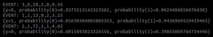
Figure 12.39: Executing a machine learning model that was imported in a Flink job from PMML
The Flink job that you have created and that now runs on your local machine is an example of a stream processing application with a machine learning model inside. The machine learning model is imported from a static PMML file and resides in the memory of the streaming job. This is an efficient way to work with models in stream processing.
Note
To access the source code for this specific section, please refer to https://packt.live/38SssNr.
By completing this exercise, you have created a stream processing job that evaluates a machine learning model in real time. The model is deserialized from the PMML format and sinks output to a local filesystem. The resulting application can predict in real time whether passengers of the Titanic would have survived the disaster of 1912. Although this real-time use case might not be so useful, you have now gained substantial practice with setting upstream processing software that can execute machine learning models.
In the next activity, you’ll build a similar stream processing application that predicts the class of Titanic passengers.
Activity 12.03: Predicting the Class of Titanic Passengers in Real Time
In this activity, we’ll create a streaming job that processes events from a local socket and produces a prediction from a machine learning model.
Note
The code for this activity can be found here:
Perform the following steps:
- Copy the model that you created in Activity12.01 (model.pkl) to the Activity12.03 directory.
- Open Jupyter and create a new Python 3 notebook in the Activity12.03 folder.
- In the first cell of the new notebook, install the sklearn2pmml library with the pip tool.
- Create a new cell and enter the import lines to start using the pickle and sklearn2pmml libraries.
- Deserialize the pickled model by using the open and pickle.load functions in a new cell.
- Export the model to the PMML format by creating a PMML pipeline, followed by a call to the sklearn2pmml method, which performs the export and writes the resulting PMML file to disk in a file called titanic_class.pmml.
- Check the contents of the generated titanic_class.pmml file by entering the following line in a new cell:
!cat titanic_class.pmml
This will produce the following output:
- Open a new Terminal window and set up Apache Flink.
- During the installation, enter the following values:
groupId: com
artifactId: titanic_class
version: 0.0.1
package: packt
This will generate a project from a template.
- Open your favorite IDE (IntelliJ IDEA, Eclipse, or another) and import the generated files by selecting pom.xml.
- Remove the BatchJob.java file since we don’t need it.
- Copy the titanic_class.pmml file that we created in Step 8 to the titanic_class/src/resources directory.
- Compile and build the code using the maven command. This produces an output that ends with BUILD SUCCESS.
- Open the pom.xml file and remove the <provided> tags in the dependencies of flink-java and flink-streaming-java. Save the file, then import the Maven changes.
- Open the StreamingJob.java file and add the import code for Flink.
- In the middle part of the file, within the main function, add code to connect the Flink job to a local socket on port 1234. Use the socketTextStream function of the existing env object (the Flink StreamExecutionEnvironment context).
- Next, add the code just after that to write (sink) the events to a file in the out directory.
- To write to a local socket, we use the Netcat tool. Test the simple code by opening a Terminal and typing the following command:
nc -l -p 1234
- Go back to your IDE and run the StreamingJob.main() method. Alternatively, run the code from the Terminal.
- In the Terminal that still runs Netcat, type a few lines of text.
- Now check the output in the out directory. You should see a subfolder with a date and time, and a file for each line that was entered in the input socket.
- Modify the pom.xml file to add the JPMML dependencies to the project, then import the Maven changes.
- Edit the StreamingJob.java file again and import jpmml.evaluator.
- Write the code to deserialize the model from PMML, loading the model in memory ready to be executed. Use the LoadingModelEvaluatorBuilder class of the JPMML library for this.
- Add a map method to the stream processing job that splits the input string, and uses the resulting string values to build a set of arguments for the machine learning model.
- Build and run the code of the Flink job together with the Netcat tool for the input socket. Enter a set of comma-separated values in the nc prompt and see which predictions are made:
1,1,13,1,56.91
0,0,81,0,0,120.96
You should get the following output:

Figure 12.41: Output of the Flink job that predicts the class of Titanic passengers
By completing this activity, you have built a streaming job with Flink that can generate predictions in real time.
Note
The solution to this activity can be found on page 670.
Summary
With this chapter, you have completed the entire book. That means you now have a thorough understanding of the infrastructure of AI systems. We have covered a tremendous number of topics in the book and supplied a great number of exercises and activities for you to follow. Let’s have a short recap of all the topics in the book.
In Chapter 1, Data Storage Fundamentals, we started with the basics – the chapter covered data storage fundamentals. You learned about AI and machine learning in general, and we used text classification as an example of a machine learning model. Chapter 2, Artificial Intelligence Storage Requirements, was about requirements and covered a great number of concepts in depth. For every data storage layer in a data lake, you learned about the specific requirements and methods to store and retrieve data at scale. We addressed security, scalability, and various other aspects of building great data-driven systems. In Chapter 3, Data Preparation, the data preparation, and processing techniques that are needed to transform data were evaluated. You learned about ETL and ELT, data cleaning, filtering, aggregating, and feature engineering. You also practiced streaming event data processing using Apache Spark.
Chapter 4, Ethics of AI Data Storage, was a less technical chapter, but perhaps even more important than the solely technical ones. The main topic was the ethics of AI storage. We explored a few famous case studies where the ethics of AI were under discussion. You learned about bias and other prejudice in data and models, which gave you a good basis to start any conversation on these topics.
In Chapter 5, Data Stores: SQL and NoSQL Databases, we did a deep dive into databases. You learned about SQL and NoSQL databases; the differences, use cases, best practices, and query languages. By doing some hands-on exercises with technologies such as MySQL, Cassandra, and MongoDB, you learned how to store data in any type of database in the historical and analytics data layers of your data lake. Chapter 6, Big Data File Formats, followed up on this by exploring the file format for big data. You practiced with CSV, JSON, Parquet, and Avro to get a broad perspective on data formats.
In Chapter 7, Introduction to Analytics Engine (Spark) for Big Data, we moved from storing data to the analysis of data. You learned a lot about Apache Spark, one of the most popular data processing engines available. This knowledge comes in handy when discussing the design of data systems, as we did in Chapter 8, Data System Design Examples. Starting from a historical perspective and following up on the requirements of Chapter 2, Artificial Intelligence Storage Requirements, this chapter explored the components of system design and addressed hardware, architecture, data pipelines, security, scaling, and much more. By completing this chapter, you gained more experience in the architecture and design of AI systems.
Chapter 9, Workflow Management for AI, contained an in-depth overview of workflow management. You practiced with several techniques, from simple Python and Bash scripts to Apache Airflow for sophisticated workflow management systems.
In Chapter 10, Introduction to Data Storage on Cloud Services (AWS), we moved on to cloud-based storage for AI systems. We used AWS to explain the concepts and technology that come with storing data in the cloud. Chapter 11, Building an Artificial Intelligence Algorithm, was a real hands-on chapter where you could practice model building and training, and finally, Chapter 12, Productionizing Your AI Applications, explored some techniques to put a machine learning model into production: building an API, running a Docker image in Kubernetes, and serializing the model to PMML to use in a data stream.
We hope that you learned a lot by reading this book. We aimed to provide a good mixture of reading content, hands-on exercises, and fun. We believe that by completing this book we have provided a solid basis for anyone who wants to build AI systems. We have drawn from our own experience, the open-source community, countless colleagues, and other people who have shared their knowledge. We hope you have enjoyed it. Please let us know about your experience with this book; we’re eager to hear from you and we’ll be happy to receive any feedback. Finally, we would like to thank you – thanks for staying with us for all these chapters, thanks for your attention, and thanks for sharing your feedback. We wish you all the best in your careers and good luck with building awesome AI systems.