
1. Data Storage Fundamentals
Activity 1.01: Creating a Text Classifier for Movie Reviews
Solution
- Create a new directory, Activity01.01, in the Chapter01 directory to store the files for this activity.
- Move the aclImdb folder to the Datasets directory.
- Open your Terminal (macOS or Linux) or Command Prompt (Windows), navigate to the Chapter01 directory, and type jupyter notebook.
- In the Jupyter notebook, click the Activity01.01 directory and create a new notebook file with a Python3 kernel.
- Import the os library and a random library, and define where our training and test data is stored using four variables, as shown in the following code:
import os
import random
dataset_train_pos_path = "../Datasets/aclImdb/train/pos/"
dataset_train_neg_path = "../Datasets/aclImdb/train/neg/"
dataset_test_pos_path = "../Datasets/aclImdb/test/pos/"
dataset_test_neg_path = "../Datasets/aclImdb/test/neg/"
We have four variables: one for training_positive, one for training_negative, one for test_positive, and one for test_negative, each pointing at the respective dataset subdirectory.
- Define a read_dataset function that reads the contents of each file in the given directory and adds these contents into a data structure, as shown in the following code:
contents_labels = [('this is the text from one '
'of the files', 'pos'),
('this is another text', 'pos')]
def read_dataset(dataset_path, label):
contents_labels = []
files = os.listdir(dataset_path)
for fn in files:
path = os.path.join(dataset_path, fn)
with open(path) as f:
s = f.read()
contents_labels.append((s, label))
return contents_labels
The read_dataset function takes a path to a dataset and a label (either pos or neg), reads the contents of each file in the given directory, and adds these contents into a data structure that is a list of tuples. Each tuple contains both the text of the file, and the label pos or neg.
- Use the read_dataset function to read each dataset into its own variable, as shown in the following code:
train_pos = read_dataset(dataset_train_pos_path, "pos")
train_neg = read_dataset(dataset_train_neg_path, "neg")
test_pos = read_dataset(dataset_test_pos_path, "pos")
test_neg = read_dataset(dataset_test_neg_path, "neg")
We have four variables in total: train_pos, train_neg, test_pos, and test_neg, each one of which is a list of tuples containing the relative text and labels.
- Combine the train_pos with train_neg datasets and test_pos with test_neg, as shown in the following code:
train = train_pos + train_neg
test = test_pos + test_neg
We combined our positive and negative examples into a single dataset so that we can train an algorithm to discriminate between the two classes.
- Use the random.shuffle function to shuffle the train and test datasets separately:
random.shuffle(train)
random.shuffle(test)
This gives us datasets where the training data is mixed up, instead of feeding all the positive and then all the negative examples to the classifier in order.
- Split each of the train and test datasets back into data and labels respectively, as shown in the following code:
train_data, y_train = zip(*train)
test_data, y_test = zip(*test)
You should have four variables again called train_data, y_train, test_data, and y_test, where the y prefix indicates that the respective array contains labels.
- Vectorize the training and test sets using TfidfVectorizer and output the dimensions of the vectors along with the vectorization time, as shown in the following code:
%%time
from sklearn.feature_extraction.text
import TfidfVectorizer
vectorizer = TfidfVectorizer()
X_train = vectorizer.fit_transform(train_data)
X_test = vectorizer.transform(test_data)
print("The dimensions of our vectors:")
print(X_train.shape)
print(«- - -»)
You should get the following output:
The dimensions of our vectors:
(25000, 74849)
- - -
CPU times: user 13.4 s, sys: 440 ms, total: 13.8 s
Wall time: 14.7 s
We import TfidfVectorizer from sklearn, initialize an instance of it, fit the vectorizer on the training data, and vectorize both the training and testing data into X_train and X_test variables respectively. Lastly, we calculate the time it takes and prints out the shape of the training vectors at the end.
- Initialize a LinearSVC model and fit it to the training data:
%%time
from sklearn.svm import LinearSVC
svm_classifier = LinearSVC()
svm_classifier.fit(X_train, y_train)
predictions = svm_classifier.predict(X_test)
You should get the following output:
CPU times: user 799 ms, sys: 63 ms, total: 862 ms
Wall time: 1.17 s
We imported the LinearSVC classifier and trained it on our training data. Then we generated predictions for every label in our test set.
- Import accuracy_score and classification_report from sklearn and calculate the results of your predictions using each:
from sklearn.metrics import accuracy_score, classification_report
print("Accuracy: {} "
.format(accuracy_score(y_test, predictions)))
print(classification_report(y_test, predictions))
You should get the following output:

Figure 1.12: Results – accuracy and full report
Now, let's see how the classifier performs when we feed it with data on different topics.
- Create two restaurant reviews as shown in the following code:
good_review = "The restaurant was really great! "
"I ate wonderful food and had "
"a very good time"
bad_review = "The restaurant was awful. "
"The staff were rude and the "
"food was horrible. I hated it"
- Now vectorize each using the same vectorizer and generate predictions for whether each one is negative or positive:
restuarant_reviews = [good_review, bad_review]
vectors = vectorizer.transform(restuarant_reviews)
print(svm_classifier.predict(vectors))
You should get the following output:
['pos' 'neg']
Note
To access the source code for this specific section, please refer to https://packt.live/3fq2Hqg.
2. Artificial Intelligence Storage Requirements
Activity 2.01: Requirements Engineering for a Data-Driven Application
Solution
- Taxi data (GPS locations, current rides), HR system data (drivers), map data, phone calls, and email records with customer interaction, website, and app input (queries for rides, page visits).
The layers for the solution are as follows:

Figure 2.16: Layers in a data-driven application
- There are daily updates from source systems: raw -> historical -> analytics layer.
There is a streaming data pipeline for events from taxis.
- The minimum set of metadata to capture is the source, owner, date, type, and the transformations that have been applied to the data records. This metadata can be used for auditing, security and consent management, and lineage reports.
- The solution will probably receive an AIC rating of 323 or higher since it contains sensitive and private data (personnel records, GPS locations, and so on). Therefore, security measures should be top-level, such as strong passwords, multi-factor authentication, and role-based access to all data.
For scalability, the raw and historical layers should be highly scalable since new data will flood into the system periodically. The analytics layer should be scalable in use since the number of concurrent users will probably grow in time. The streaming data layer should be scalable to some extent in order to keep up with incoming event data for when the number of taxis increases. The model development environment should be scalable in various aspects: data, number of users, and performance.
The availability of the system should be high (99.9% or better) for the streaming data layer since running the new system (and therefore the business strategy) depends on the analysis of that data. Other layers can have lower availability rates since they are less mission-critical.
- Time travel is needed for historical reports and audits, and for historical analysis by data analysts and data scientists.
Retention is important in the raw and historical layers to comply with laws and regulations, in the analytics layer to retain good performance, and in the streaming data layer to limit the amount of data that is being processed at any given moment.
The locality of the data becomes important once the taxi company expands to other regions/countries.
- There is a trade-off between costs and quality. A certain minimum level of quality should be in place; for example, software development principles that ensure a high level of maintainability.
- The model development layer should import data from the raw data layer, the historical data layer, the analytics layer, and the streaming data layer. It must have enough processing power (memory and processing in the form of CPUs and/or GPUs) to train the models for forecasting.
3. Data Preparation
Activity 3.01: Using PySpark for a Simple ETL Job to Find Netflix Shows for All Ages
Solution
- Create a directory called Activity03.01 in the Chapter03 directory to store the files for this activity.
- Open your Terminal (macOS or Linux) or Command Prompt (Windows), navigate to the Chapter03 directory, and type jupyter notebook.
- Select the Activity03.01 directory, then click New -> Python3 to create a new Python 3 notebook.
- If you have done Exercise 3.02, Building an ETL Job Using Spark, PySpark is already installed on your local machine. If not, install PySpark with the following lines:
import sys
!conda install --yes --prefix {sys.prefix}
-c conda-forge pyspark
- Connect to a Spark cluster or a local instance using the following code:
from pyspark.sql import SparkSession
from pyspark.sql.functions import col, split, size
spark = SparkSession.builder.appName("Packt").getOrCreate()
- Load and show the contents of the dataset using the following code:
data = spark.read.csv(
'../../Datasets/netflix_titles_nov_2019.csv',
header='true')
data.show()
Note
We read the data from a relative file path. You can also copy the CSV file to the same Activity03.01 directory and use netflix_titles_nov_2019.csv as the path.
You should get the following output:

Figure 3.23: The contents of the CSV file
- Apply the data.filter() function to filter the shows with a rating of TV-G and TV-Y, as shown in the following code:
movies = data.filter((col('type') == 'TV Show') &
((col('rating') == 'TV-G') |
(col('rating') == 'TV-Y')))
movies.show()
You should get the following output:

Figure 3.24: The contents of the file with TV shows filtered by rating
- Add the count_lists column, which contains the number of lists that are in the listed_in column, as shown in the following code:
transformed = movies.withColumn('count_lists',
size(split(movies['listed_in'], ',')))
- Select a subset of columns using the following code:
selected = transformed.select('title', 'cast',
'rating', 'release_year', 'duration',
'count_lists', 'listed_in', 'description')
- View the data in the selected column using the following code:
selected.show()
You should get the following output:
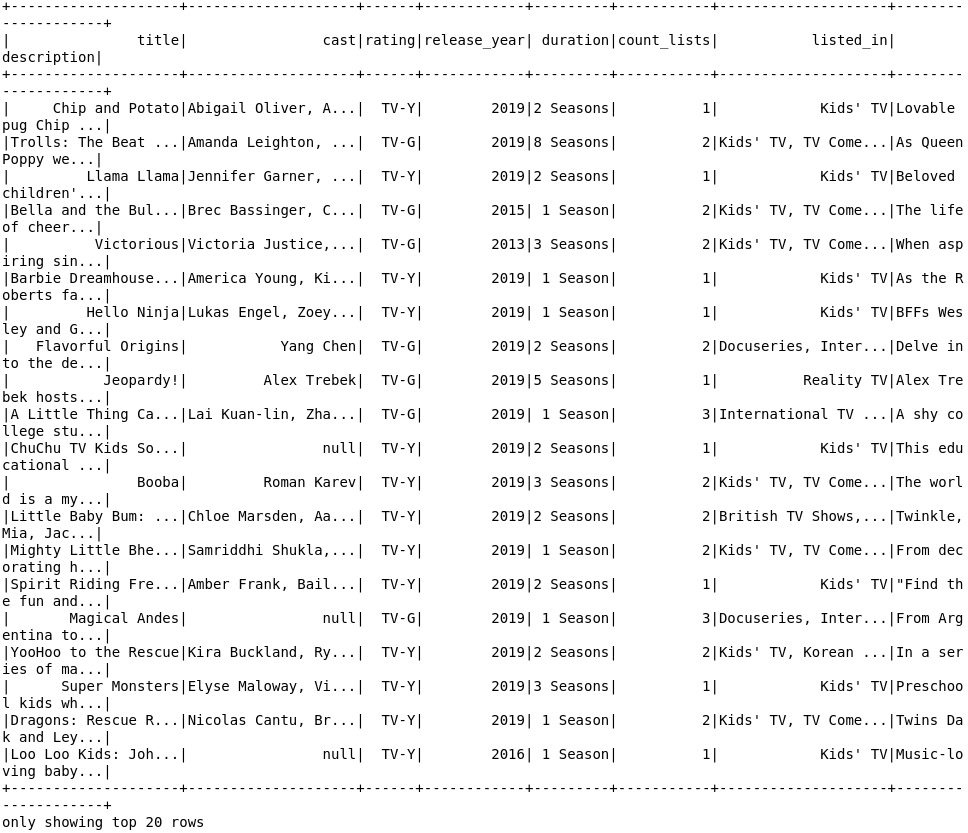
Figure 3.25: The contents of the file with the selected columns
- Write the contents of our still in-memory DataFrame to the transformed2 directory using the following code:
selected.write.csv('transformed2', header='true')
Note
Alternatively, we can add the complete code of the ETL process so far in a Python script and run it through the Terminal (macOS or Linux) or Command Prompt (Windows). We have created the same spark_etl.py Python script at the following location: https://packt.live/2ZqQxb9.
- Open the CSV file in the transformed2 directory in Jupyter Notebook using the following command:
# note: the filename ('part-....') will differ
#in your local machine
!head transformed2/part-00000-a9837c96-549d-4a8c-981a-
cae147e36801-c000.csv
You should get the following output:
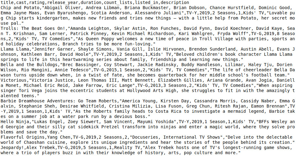
Figure 3.26: CSV file in the transformed2 directory
Note
To access the source code for this specific section, please refer to https://packt.live/3iXSinP.
Activity 3.02: Counting the Words in a Twitter Data Stream to Determine the Trending Topics
Solution
- Create a new Python file in your favorite editor (for example, PyCharm or VS Code) or a Jupyter Notebook and name it spark_twitter.py or spark_twitter.ipynb.
- If you have done Exercise 3.02, Building an ETL Job Using Spark, PySpark is already installed on your local machine. If not, install PySpark with the following lines:
import sys
!conda install --yes --prefix {sys.prefix}
-c conda-forge pyspark
- We first have to connect to a Spark cluster or a local instance. Enter the following lines in the file, notebook, or Python shell:
from pyspark.sql import SparkSession
from pyspark.sql.functions import from_json, window,
to_timestamp, explode, split, col
from pyspark.sql.types import StructType, StructField, StringType
- Enter the following line to create a Spark session:
spark = SparkSession.builder.appName('Packt').getOrCreate()
- To connect to socket on localhost, enter the following line:
raw_stream = spark.readStream.format('socket').option(
'host', 'localhost').option('port', 1234).load()
- We'll define the JSON schema and add the string format that Twitter uses for its timestamps:
tweet_datetime_format = 'EEE MMM dd HH:mm:ss ZZZZ yyyy'
schema = StructType([StructField('created_at',
StringType(), True),
StructField('text', StringType(), True)])
- We can now convert the JSON strings with the from_json PySpark function:
tweet_stream = raw_stream.select(from_json('value', schema).alias('tweet'))
- Convert the field that contains the event time to a timestamp with the to_timestamp function and split the text of the tweets in words by using the explode and split functions as shown in the following code:
timed_stream = tweet_stream.select(
to_timestamp('tweet.created_at', tweet_datetime_format).alias('timestamp'),
explode(
split('tweet.text', ' ')
).alias('word'))
- Create a tumbling window of 10 minutes with groupBy(window(…)) and add a watermark that ensures that we have a slack of 1 minute before the window evaluates. Make sure to group the tweets in two fields – the window, and the words of the tweets:
windowed = timed_stream
.withWatermark('timestamp', '1 minute')
.groupBy(window('timestamp', '10 minutes'), 'word')
- Specify the evaluation function of the window that is a count of all the words in the window as shown in the following code:
counts_per_window = windowed.count().orderBy(['window', 'count'], ascending=[0, 1])
- Send the output of the stream to the console and start executing the stream with the awaitTermination function:
query = counts_per_window.writeStream.outputMode('complete')
.format('console').option("truncate", False).start()
query.awaitTermination()
You should get the following output:

Figure 3.27: Spark Structured Streaming job that connects to Twitter
Note
To access the source code for this specific section, please refer to https://packt.live/3iX0ODx.
4. Ethics of AI Data Storage
Activity 4.01: Finding More Latent Prejudices
Solution
- Create the Activity04.01 directory in the Chapter04 directory to store the files for this activity.
- Open your Terminal (macOS or Linux) or Command Prompt (Windows), navigate to the Chapter04 directory, and type jupyter notebook.
- In the Jupyter Notebook, click the Activity04.01 directory and create a new notebook file with the Python3 kernel.
- Create a list of at least 16 words that you think might have a positive or negative prejudice:
words = """sporty
nerdy
employed
unemployed
clever
stupid
latino
asian
caucasian
disabled
pregnant
introvert
extrovert
politician
florist
CEO"""
In the previous code, we added 16 words to our list.
- Define the same classification model that we used in previous exercises:
import spacy
nlp = spacy.load('en_core_web_lg')
def polarity_good_vs_bad(word):
"""Returns a positive number if a word is closer to good than it is to bad, or a negative number if vice versa
IN: word (str): the word to compare
OUT: diff (float): positive if the word is closer to good, otherwise negative
"""
good = nlp("good")
bad = nlp("bad")
word = nlp(word)
if word and word.vector_norm:
sim_good = word.similarity(good)
sim_bad = word.similarity(bad)
diff = sim_good - sim_bad
diff = round(diff * 100, 2)
return diff
else:
return None
In the preceding code, we defined our basic sentiment classification model again. It takes in a word and checks whether it is closer to good or closer to bad.
- Before running the code, guess whether each of the words you chose will be classified as a positive or negative word:
# Guesses
"""sporty : POS
nerdy : NEG
employed : POS
unemployed : NEG
clever : POS
stupid : NEG
latino : NEG
asian : NEG
caucasian : POS
disabled : NEG
pregnant : NEG
introvert : NEG
extrovert : POS
politician : NEG
florist : POS
CEO: NEG"""
In the preceding code, we added POS (positive) or NEG (negative) next to the words in our list, guessing their polarity.
- Run the classifier on the word list and see how close your predictions were, as shown in the following code:
for word in words.split(" "):
print(word, polarity_good_vs_bad(word))
You should get the following output:
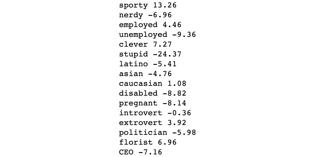
Figure 4.17: The polarity scores for each word in our new list
In the preceding code, we looped through all the words in our list and calculated their polarity. We can see that our predictions were right in all cases.
Note
To access the source code for this specific section, please refer to https://packt.live/2Zqk84p.
5. Data Stores: SQL and NoSQL Databases
Activity 5.01: Managing the Inventory of an E-Commerce Website Using a MySQL Query
Solution
- Open a Terminal and run the MySQL client using the following command, based on your OS:
Windows:
mysql
Linux:
sudo mysql
macOS:
mysql
- Create and select the PacktFashion database using the following commands:
Create database PacktFashion;
use PacktFashion;
You should get the following output:

Figure 5.71: Created and selected database for operation
Next, we will create the tables as per the data model.
- Create the manufacturer table based on the data model, as shown in the following query:
CREATE TABLE manufacturer (m_id INT,
m_name TEXT,
m_created_at TIMESTAMP,
PRIMARY KEY (m_id)
);
- Create the products table based on the data model, as shown in the following query:
CREATE TABLE products (p_id INT,
p_name TEXT,
p_buy_price FLOAT,
p_manufacturer_id INT,
p_created_at TIMESTAMP,
PRIMARY KEY (p_id),
FOREIGN KEY (p_manufacturer_id)
REFERENCES manufacturer(m_id)
ON DELETE CASCADE
);
Declaring the ON DELETE CASCADE command will force MySQL to delete the data from the child table when any parent key is deleted. For example, if any m_id entry is deleted from the manufacturer table, then all the rows matching the p_manufacturer_id column will also be deleted from the products table.
- Create the sales table based on the data model, as shown in the following query:
CREATE TABLE sales (s_id INT,
p_id INT,
s_sale_price FLOAT,
s_profit FLOAT,
s_created_at TIMESTAMP,
PRIMARY KEY (s_id),
FOREIGN KEY (p_id)
REFERENCES products(p_id)
ON DELETE CASCADE
);
- Create the location table based on the data model, as shown in the following query:
CREATE TABLE location (loc_id INT,
loc_name TEXT,
loc_created_at TIMESTAMP,
PRIMARY KEY (loc_id)
);
- Create the status table based on the data model, as shown in the following query:
CREATE TABLE status (status_id INT,
status_name TEXT,
status_created_at TIMESTAMP,
PRIMARY KEY (status_id)
);
- Create the inventory table based on the data model, as shown in the following query:
CREATE TABLE inventory (inv_id INT,
inv_loc_id INT,
inv_p_id INT,
inv_status_id INT,
inv_created_at TIMESTAMP,
PRIMARY KEY (inv_id),
FOREIGN KEY (inv_loc_id)
REFERENCES location(loc_id)
ON DELETE CASCADE,
FOREIGN KEY (inv_p_id)
REFERENCES products(p_id)
ON DELETE CASCADE,
FOREIGN KEY (inv_status_id )
REFERENCES status(status_id)
ON DELETE CASCADE
);
Now that the structure is ready, we will insert data into the tables.
- Insert the necessary data into the manufacturer table using the INSERT INTO command, as shown in the following query:
INSERT INTO manufacturer(m_id, m_name, m_created_at)
VALUES
(1,"Z-1", now()),
(2,"XIMO", now()),
(3,"NY", now());
- Insert the necessary data into the products table using the INSERT INTO command, as shown in the following query:
INSERT INTO products(p_id, p_name, p_buy_price, p_manufacturer_id, p_created_at)
VALUES
(1, 'Z-1 Running shoe', 34, 1, now()),
(2, 'XIMO Trek shirt', 15, 2, now()),
(3, 'XIMO Trek shorts', 18, 2, now()),
(4, 'NY cap', 18, 3, now());
- Insert the necessary data into the sales table using the INSERT INTO command, as shown in the following query:
INSERT INTO sales(s_id, p_id, s_sale_price, s_profit, s_created_at)
VALUES
(1,2,18,3,now()),
(2,3,20,2,now()),
(3,3,19,1,now()),
(4,1,40,6,now()),
(5,1,34,0,now());
- Insert the necessary data into the location table using the INSERT INTO command, as shown in the following query:
INSERT INTO location(loc_id, loc_name, loc_created_at)
VALUES
(1, 'California', now()),
(2, 'London', now()),
(3, 'Prague', now());
- Insert the necessary data into the status table using the INSERT INTO command, as shown in the following query:
INSERT INTO status(status_id, status_name, status_created_at)
VALUES
(1, 'IN', now()),
(2, 'OUT', now());
- Insert the necessary data into the inventory table using the INSERT INTO command, as shown in the following query:
INSERT INTO inventory(inv_id,
inv_loc_id,
inv_p_id,
inv_status_id,
inv_created_at)
VALUES
(1,1,3,1,now()),
(2,3,4,1,now()),
(3,2,2,2,now()),
(4,3,2,2,now()),
(5,1,1,2,now());
- View the manufacturer table's data using the SELECT query:
SELECT * FROM manufacturer;
You should get the following output:

Figure 5.72: SELECT query output from the manufacturer table
- View the products table's data using the SELECT query:
SELECT * FROM products;
You should get the following output:

Figure 5.73: SELECT query output from the products table
- View the sales table's data using the SELECT query:
SELECT * FROM sales;
You should get the following output:

Figure 5.74: SELECT query output from the sales table
The formula that's used for calculating profit is (sale price – buy price). In each record, we can see that the sales price is different for the same product. It is assumed that the selling prices are different based on various sale offers.
- View the location table's data using the SELECT query:
SELECT * FROM location;
You should get the following output:

Figure 5.75: SELECT query output from the location table
- View the status table's data using the SELECT query:
SELECT * FROM status;
You should get the following output:

Figure 5.76: SELECT query output from the status table
- View the inventory table's data using the SELECT query:
SELECT * FROM inventory;
You should get the following output:

Figure 5.77: SELECT query output from the inventory table
This inventory table defines the product inventory where inv_p_id refers to p_id from the products table, inv_status_id refers to status_id from the status table, and inv_loc_id refers to loc_id from the location table. Let's understand this better using a third row where inv_id (inventory ID) is 3. This can be declassified as stating that the XIMO Trek Shirt product (that is, inv_p_id is 2) is not available (that is, inv_status_id is 2) in the London warehouse (inv_loc_id is 2).
- Find the total number of products in the inventory table using the count function and a JOIN clause, as shown in the following query:
SELECT count(inventory.inv_p_id) as total_in_stock_products
FROM inventory
JOIN status
ON status.status_id=inventory.inv_status_id
WHERE status.status_name='IN';
You should get the following output:

Figure 5.78: Table showing the total of in-stock products
We need to join the inventory and status tables on inv_status_id and status_id and count the total products available with Status_name='IN' in the products table.
- Find the total number of products not in the inventory using the count function and a JOIN clause, as shown in the following query:
SELECT count(inventory.inv_p_id) as total_in_stock_products
FROM inventory
JOIN status
ON status.status_id=inventory.inv_status_id
WHERE status.status_name='OUT';
You should get the following output:

Figure 5.79: Table showing the total of out-of-stock products
This scenario is similar to the previous step. In this step, we are filtering for the 'OUT' status.
- Find the status of the XIMO Trek shirt product for the Prague location, as shown in the following query:
SELECT status.status_name as status
FROM inventory, status, products, location
WHERE status.status_id=inventory.inv_status_id
AND products.p_id = inventory.inv_p_id
AND location.loc_id = inventory.inv_loc_id
AND products.p_name='XIMO Trek shirt'
AND location.loc_name='Prague';
You should get the following output:

Figure 5.80: Table showing the status of the product
We select status_name from the status table and apply conditions to other tables, that is, inventory, products, and location. Let's join on the primary key and foreign keys from the inventory, status, products, and location tables. Then, we'll filter for the location as 'Prague' and the product name as 'XIMO Trek shirt'.
Note
To access the source code for this specific section, please refer to https://packt.live/2ZpQpbz.
Activity 5.02: Data Model to Capture User Information
Solution
- Open a Terminal and start a MongoDB shell:
$mongo
- Create a database called PacktFashion through the use query:
use PacktFashion
You should get the following output:
switched to db PacktFashion
In MongoDB, you can start using the database directly without creating it. It will be created when you create a collection in it.
- Create a products collection, as shown in the following query:
db.createCollection("products")
You should get the following output:
{ "ok" : 1 }
- Insert the data into the products collection, as shown in the following query:
todayDate=new Date()
products=[{
"p_name": "XIMO Trek shirt",
"p_manufacturer": "XIMO",
"p_buy_price": 15,
"p_created_at": todayDate,
"sales": [
{
"s_sale_price": 30,
"s_profit": 15,
"p_created_at": todayDate,
},
{
"s_sale_price": 18,
"s_profit": 3,
"p_created_at": todayDate
},
{
"s_sale_price": 20,
"s_profit": 5,
"p_created_at": todayDate
},
{
"s_sale_price": 15,
"s_profit": 0,
"p_created_at": todayDate
}
]
},
{
"p_name": "XIMO Trek shorts",
"p_manufacturer": "XIMO",
"p_buy_price": 18,
"p_created_at": todayDate,
"sales": [
{
"s_sale_price": 22,
"s_profit": 4,
"p_created_at": todayDate,
},
{
"s_sale_price": 18,
"s_profit": 0,
"p_created_at": todayDate
},
{
"s_sale_price": 20,
"s_profit": 2,
"p_created_at": todayDate
}
]
},
{
"p_name": "NY cap",
"p_manufacturer": "NY",
"p_buy_price": 18,
"p_created_at": todayDate,
"sales": [
{
"s_sale_price": 20,
"s_profit": 2,
"p_created_at": todayDate,
},
{
"s_sale_price": 21,
"s_profit": 3,
"p_created_at": todayDate
},
{
"s_sale_price": 19,
"s_profit": 1,
"p_created_at": todayDate
}
]
}
]
- Insert the products object as a document into the collection, as shown in the following query:
db.products.insert(products)
You should get the following output:
WriteResult({ "nInserted" : 1 })
We have successfully inserted the product and sales data into the database. Now, we would like to track the user's actions. To do this, we will need two collections, users and user_logs, as per the data model.
- Create and insert data into the users collection, as shown in the following query:
users=[
{
"name":"Max",
"u_created_at":todayDate
},
{
"name":"John Doe",
"u_created_at":todayDate
},
{
"name":"Roger smith",
"u_created_at":todayDate
},
];
- Create and enter the necessary logs into the user_logs collection, as shown in the following query:
user_logs=[
{
user_id:"Max",
product_id:"XIMO Trek shirt",
action:"bought",
ul_crated_at:todayDate
},
{
user_id:"John Doe",
product_id:"NY cap",
action:"bought",
ul_crated_at:todayDate
},
{
user_id:"Roger smith",
product_id: "XIMO Trek shorts",
action:"bought",
ul_crated_at:todayDate
}
];
- Insert the users object as a document into the collection, as shown in the following query:
db.users.insert(users);
You should get the following output:
WriteResult({ "nInserted" : 1 })
- Insert the user_logs object as a document into the collection, as shown in the following query:
db.user_logs.insert(user_logs);
You should get the following output:
WriteResult({ "nInserted" : 1 })
- Join the users and user_logs collections using an aggregation pipeline, as shown in the following query:
var user_logs_aggregate_pipeline = [
{ $lookup:
{
from: "users",
localField: "user_id",
foreignField: "name",
as: "users"
}
},
{
$lookup:
{
from: "products",
localField: "product_id",
foreignField: "p_name",
as: "products"
}
},
{
"$unwind":"$users"
},
{
"$project": {
"user":"$users.name",
"product":"$products.p_name",
"action":"$action"
}
}
];
We have joined three collections of products, users, and user_logs using the $lookup operator of the aggregate pipeline. Once the joining is done, we exploded the products and users arrays using the $unwind operator. You can perform various types of aggregation just to get comfortable with it before diving into more complex usage.
- Generate the report of user logs using the JavaScript array object with the aggregate function, as shown in the following query:
db.user_logs.aggregate(user_logs_aggregate_pipeline).pretty()
You should get the following output:

Figure 5.81: Using $lookup to join the collections
Note
To access the source code for this specific section, please refer to https://packt.live/38T4b9X.
Activity 5.03: Managing Customer Feedback Using Cassandra
Solution
- Launch the Cassandra CLI based on your OS, as follows:
Windows:
Open Cassandra CLI application
Linux:
root@ubuntu: -$ cqlsh
macOS:
MyMac:~ root$ cqlsh
You should get the following output:
cqlsh>
- Create and select the fashionmart keyspace, as shown in the following query:
CREATE KEYSPACE fashionmart
WITH replication = {'class':'SimpleStrategy', 'replication_factor' : 3};
use fashionmart;
- Create a COLUMNFAMILY called feedback_logs, as shown in the following query:
CREATE COLUMNFAMILY feedback_logs(
fl_id int PRIMARY KEY,
fl_feedback text,
fl_location text,
fl_created_at timestamp);
- Check whether the feedback_logs column family was created in the fashionmart keyspace using the following query:
describe tables;
You should get the following output:
feedback_logs user
- Insert the records as batches into the feedback_logs column family, as shown in the following query:
BEGIN BATCH
INSERT INTO feedback_logs(fl_id, fl_feedback, fl_location, user_id, fl_created_at)
VALUES(1, 'Great website', 'London', 3, '2019-10-30 12:05:00+0000');
INSERT INTO feedback_logs(fl_id, fl_feedback, fl_location, user_id, fl_created_at)
VALUES(2, 'Good work', 'Seattle', 2, '2019-10-03 12:05:00+0000');
INSERT INTO feedback_logs(fl_id, fl_feedback, fl_location, user_id, fl_created_at) VALUES(3, 'Amazing', 'Seattle', 2, '2019-11-04 11:05:00+0000');
INSERT INTO feedback_logs(fl_id, fl_feedback, fl_location, user_id, fl_created_at) VALUES(4, 'Not so good', 'Hong Kong', 1, '2019-11-04 11:05:00+0000');
INSERT INTO feedback_logs(fl_id, fl_feedback, fl_location, user_id, fl_created_at) VALUES(, 'Informative website', 'Shanghai', 1, '2018-11-04 11:05:00+0000');
INSERT INTO feedback_logs(fl_id, fl_feedback, fl_location, user_id, fl_created_at) VALUES(5, 'Great website', 'London', 1, '2019-10-30 12:05:00+0000');
INSERT INTO feedback_logs(fl_id, fl_feedback, fl_location, user_id, fl_created_at) VALUES(6, 'Good work', 'Seattle', 4, '2019-10-03 12:05:00+0000');
INSERT INTO feedback_logs(fl_id, fl_feedback, fl_location, user_id, fl_created_at) VALUES(7, 'Informative website', 'Shanghai', 2, '2018-11-04 11:05:00+0000');
APPLY BATCH;
- View the feedback_logs column family's data using the SELECT query:
SELECT * FROM feedback_logs;
You should get the following output:

Figure 5.82: The feedback_logs column family data
- Calculate the total amount of feedback, as shown in the following query:
SELECT COUNT(fl_id) AS total_feedback
FROM feedback_logs;
You should get the following output:

Figure 5.83: Showing total visits
Note
To access the source code for this specific section, please refer to https://packt.live/2Ok942r.
6. Big Data File Formats
Activity 6.01: Selecting an Appropriate Big Data File Format for Game Logs
Solution
- In the Chapter06 directory, create the Activity06.01 directory to store the files for this activity.
- Move the session_log file into the Chapter06/Data directory.
- Open your Terminal (macOS or Linux) or Command Prompt window (Windows), move to the installation directory, and open the Spark shell in it using the following command:
spark-shell --packages org.apache.spark:spark-avro_2.11:2.4.5
You should get the following output:

Figure 6.27: Spark shell
By using this command, the Spark shell will be launched and we will now load the dataset from the CSV file.
- Load the session_log.csv dataset:
val df_ses_log_csv = spark.read.options(Map("inferSchema"- >"true","delimiter"->",","header"- >"true")).csv("F:/Chapter06/Data/session_log.csv")
Note
Update the input path of the file according to your local file path throughout the exercise.
You should get the following output:
df_ses_csv: org.apache.spark.sql.DataFrame = [user_id: string, event_date: string … 3 more fields]
Here, we have loaded the dataset from the CSV file with an explicit option of a delimiter (or value separator), and the header argument set to true because the dataset contains the schema or column names. This will result in a DataFrame.
- Show the CSV file using the following command:
df_ses_log_csv.show(false)
Note
Owing to the size of the data, the commands in this activity can take up to a few minutes to execute.
You should get the following output:

Figure 6.28: Displaying the DataFrame
This will display the first 20 rows from the DataFrame. The false argument represents the width of the columns shown to match the complete raw value.
- Convert the CSV file into the Avro file format and verify the file size as shown in the following code:
df_ses_log_csv.write.format("avro").save("F:/Chapter06/Data/session_log.avro")
A file is created of the following size:
Output file size: 454 MB
This command will convert the DataFrame(that loaded the CSV file) and save it into the Avro file format. The time taken to execute this command will vary as per the size of the data. Let's convert the data to the ORC format now.
- Convert the CSV file into the ORC file format and verify the file size as shown in the following code:
df_ses_log_csv.write.orc("F:/Chapter06/Data/session_log.orc")
A file is created of the following size:
Output file size: 182 MB
This command will convert the DataFrame(that loaded the CSV file) and save it in the ORC file format. The time taken to execute this command will vary as per the size of the data. Let's convert the data into the Parquet format now.
- Convert the CSV file into the Parquet file format and verify the file size as shown in the following code:
df_ses_log_csv.write.parquet(«F:/Chapter06/Data/session_log.parquet»)
A file is created of the following size:
[Output file size: 115 MB]
This command will convert the DataFrame(that loaded the CSV file) and save it in the Parquet file format. The time taken to execute this command will vary as per the size of the data. Now, let's measure the query performance.
- Read the Parquet file through the DataFrame as shown in the following code:
var df_ses_log_parquet =
spark.read.parquet(«F:/Chapter06/Data/session_log.parquet»)
You should get the following output:
df_ses_log_parquet: org.apache.spark.sql.DataFrame =
[user_id: string, event_date: string … 3 more fields]
- Read the ORC file through the DataFrame as shown in the following code:
var df_ses_log_orc = spark.read.orc("F:/Chapter06/Data/session_log.orc")
You should get the following output:
df_ses_log_orc: org.apache.spark.sql.DataFrame = [user_id: string, event_date: string … 3 more fields]
- Read the Avro file through the DataFrame as shown in the following code:
var df_ses_log_avro = spark.read.format("avro").load("F:/Chapter06/Data/session_log.avro")
You should get the following output:
df_ses_log_avro: org.apache.spark.sql.DataFrame = [user_id: string, event_date: string … 3 more fields]
We have created three DataFrames by loading the data from our Parquet, Avro, and ORC files. Now we will create a function to measure the execution time.
- Create a function to measure the execution time as follows:
// Function for time consumption
def time[A](f: => A) = {
val s = System.nanoTime
val ret = f
println("Time: "+(System.nanoTime-s)/1e6+" ms")
ret
}
In this step, we have create a time-measuring function that will take the query that needs to be executed as an input. Let's run the performance query to measure the efficiency of each file format.
- Execute the count query within the time function for all three DataFrames as shown in the following code:
time{df_ses_log_avro.groupBy("session_nb").count()}
time{df_ses_log_parquet.groupBy("session_nb").count()}
time{df_ses_log_orc.groupBy("session_nb").count()}
You should get the following output:
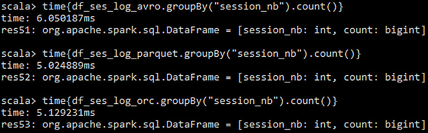
Figure 6.29: Time consumed for count queries by each format
In this step, we have executed the count query over the DataFrames created in the previous steps. We can observe that the ORC and Parquet files have nearly the same time-efficiency over this query. Let's execute a few complex queries.
- Create a table from the DataFrames as shown in the following code:
//Parquet
df_ses_log_parquet.createOrReplaceTempView(«session_log_parquet»)
//ORC
df_ses_log_orc.createOrReplaceTempView(«session_log_orc»)
//AVRO
df_ses_log_avro.createOrReplaceTempView(«session_log_avro»)
By creating a table from the DataFrames, we can execute SQL syntax queries over the same dataset. Let's now execute the queries.
- Execute a GROUP BY query over the created tables as follows:
// Defining sql query as a variable
val p_yr_query = "Select count(Year),Year from (Select SUBSTRING(event_date,7,10) as Year from session_log_parquet) GROUP BY Year"
val o_yr_query = "Select count(Year),Year from (Select SUBSTRING(event_date,7,10) as Year from session_log_orc) GROUP BY Year"
val a_yr_query = "Select count(Year),Year from (Select SUBSTRING(event_date,7,10) as Year from session_log_avro) GROUP BY Year"
// Executing the query inside the time function
time{spark.sql(p_yr_query)}
time{spark.sql(o_yr_query)}
time{spark.sql(a_yr_query)}
You should get the following output:

Figure 6.30: Time consumed by a GROUP BY query
In this step, we have executed a complex GROUP BY query with a SUBSTRING function over all the DataFrames. And again, the ORC and Parquet files have nearly the same time-efficiency over this query.
We can conclude from the results that the Parquet file format has the highest compression for our dataset, and ORC has the quickest query response. However, the difference in operational efficiency does not have a high delta.
Along with technical specifications, there are a few other considerations before finalizing your choice of file format. These include scopes such as the current environment or platform, the cost and time of adopting the new environment, and the impact of such a change on the business. Let's include the technology stack of the company in our decision making.
- Consolidating these factors into a single selection, and taking into consideration the existing technology stack, which is Spark and Cloudera, which have seamless support for Parquet, your report will likely contain a preference for Parquet over the ORC file format.
Note
To access the source code for this specific section, please refer to https://packt.live/3gU6yMu.
7. Introduction to Analytics Engine (Spark) for Big Data
Activity 7.01: Exploring and Processing a Movie Locations Database by Using Spark's Transformations and Actions
Solution
- The first step involves logging in to the COMMUNITY EDITION of Databricks.
- Upload the file you have downloaded, Film_Locations_in_San_Francisco.csv, into Databricks:

Figure 7.33: Uploading the file
- Read the CSV file to a DataFrame:
from pyspark.sql.functions import desc
# File location and type
file_location = "/FileStore/tables/Film_Locations_in_San_Francisco.csv"
file_type = "csv"
# The applied options are for CSV files. For other file types, these will be ignored.
dataTable = spark.read.format(file_type)
.option("inferSchema", "true")
.option("header", "true")
.option("sep", ",")
.load(file_location)
display(dataTable)
dataTable.printSchema()
You should get the following output:

Figure 7.34: View of the data read
Note
As the output was long, the view is truncated for ease of representation.
We read the CSV file into a DataFrame called dataTable by using the spark.read.format() function. The function takes in several arguments, we specify the delimiter as a comma (,), specify the file path, specify the first row as the header of the DataFrame using header=true, and the data types can be inferred from the samples of the DataFrame by setting inferSchema = true.
- Rename the columns with no spaces between the words, as shown in the following code:
newcolnames = ['Title','ReleaseYear', 'Locations',
'FunFacts', 'ProductionCompany',
'Distributor', 'Director', 'Writer',
'Actor1', 'Actor2', 'Actor3']
for old,new in zip(dataTable.columns, newcolnames):
dataTable = dataTable.withColumnRenamed(old,new)
display(dataTable)
You should get the following output:
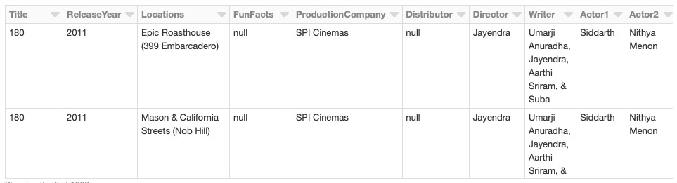
Figure 7.35: Snapshot of the view created with the renamed column
Note
As the output was long, the view is truncated for ease of representation.
We remove the space in the column names by renaming them using the withColumnRenamed function. We do this by creating a list of new column names, newcolnames, and using the new list to rename the old list of columns.
- Find the recent movies released in or after 2015 using the following code:
#finding the recent movies released after 2015
recentMovies= dataTable.filter(dataTable.ReleaseYear >= 2015)
display(recentMovies)
You should get the following output:
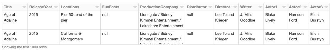
Figure 7.36: Recently released movies (released in 2015 or later) shot in SFO
Note
As the output was long, the view is truncated for ease of representation.
We use the filter function to find the list of movies released in the year 2015 or later.
- Find and show the popular locations of recently released movies shot in SFO using the following code:
#group by locations and find the count
recentLocations = recentMovies.groupby('Locations')
.count().sort(desc("count"))
display(recentLocations)
You should get the following output:

Figure 7.37: Popular locations of recently released movies shot in SFO
We find the popular location of recently released movies by aggregating on a writer by using the groupby and count functions. We then sort in descending order with the help of the sort(desc("count")) function.
- Find and show the top three popular locations in recent movies shot in SFO using the following code:
display(recentLocations.take(3))
You should get the following output:

Figure 7.38: Top three popular locations of recently released movies shot in SFO
We find and display the top three rows from the recentLocations DataFrame by using the take function, with an argument of 3.
- Find and show the most popular location for the recent movies shot in SFO using the following code:
recentLocations.first()
display(recentLocations.take(1))
You should get the following output:

Figure 7.39: The most popular location of recently released movies shot in SFO
We find and display the topmost row from the recentLocations DataFrame by using the first() function.
- Show the popular writers of recently released movies shot in SFO using the following code:
recentWriters = recentMovies.groupby('Writer').count().sort(desc("count"))
display(recentWriters)
You should get the following output:
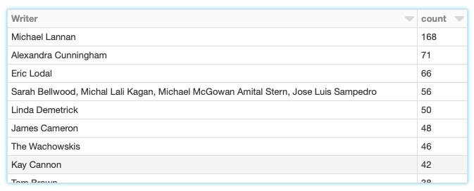
Figure 7.40: Popular writers of recently released movies shot in SFO
Note
As the output was long, the view is truncated for ease of representation.
We find the popular writers of recently released movies by aggregating on a writer by using the groupby and count functions. We then sort in descending order with the help of the sort(desc("count")) function.
- Show the top three popular writers of recently released movies shot in SFO using the following code:
display(recentWriters.take(3))
You should get the following output:
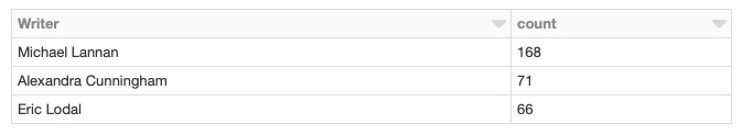
Figure 7.41: Top three popular writers of recently released movies shot in SFO
We find and display the top three rows from the recentWriters DataFrame by using the take function, with an argument of 3.
- Find and show the most popular writer of recently released movies shot in SFO using the following code:
recentWriters.first()
display(recentWriters.take(1))
You should get the following output:
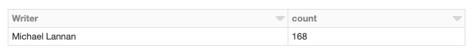
Figure 7.42: The most popular writer of recently released movies shot in SFO
We find and display the topmost row from the recentWriters DataFrame by using the first() function.
Note
To access the source code for this specific section, please refer to https://packt.live/2OoDtN2.
8. Data System Design Examples
Activity 8.01: Building the Complete System with Pipelines and Queues
Solution
- Import the random and time standard libraries, as well as the Queue and Thread classes from their respective modules:
from queue import Queue
from threading import Thread
import random
import time
We imported the modules that we will use to design our next mock system.
- Initialize the mock dataset and put it into a queue, as shown in the following query:
urls = ['url1-', 'url1-', 'url2-', 'url3-', 'url4-',
'url5-', 'url6-', 'url7-', 'url8-', 'url9-', 'url10-']
seen = set()
url_queue = Queue()
for url in urls:
url_queue.put(url)
We created 11 mock URLs and a seen set to find duplicates. We then created a queue for our URLs and added each URL to the queue.
- Set up queues for each of the components, as shown in the following query:
scraped_queue = Queue()
cleaned_queue = Queue()
deduplicated_queue = Queue()
insights_queue = Queue()
decisions_queue = Queue()
We initialized Queue() objects for each component to push to when done.
- Define the scraper, cleaner, and deduplicator modules, just like we did in Exercise 8.02, Adding Queues to a System to Make It Highly Available:
def scraper():
while True:
time.sleep(random.randrange(0,2))
url = url_queue.get()
print("Scraping {}".format(url))
scraped_queue.put(url[3:])
def cleaner():
while True:
time.sleep(random.randrange(2,4))
raw = scraped_queue.get()
print("Cleaning {}".format(raw))
cleaned_queue.put(raw.replace("-", ""))
def deduplicator():
while True:
time.sleep(random.randrange(4,6))
cleaned = cleaned_queue.get()
print("Deduplicating {}".format(cleaned))
if cleaned not in seen:
deduplicated_queue.put(cleaned)
seen.add(cleaned)
We defined each of these functions in the same way we did previously.
- Define the analyzer module, as shown in the following query:
def analyzer():
while True:
time.sleep(random.randrange(1,4))
unique = deduplicated_queue.get()
print(«Analyzing {}».format(unique))
n = int(unique)
if n % 2 == 0:
insights_queue.put(-n)
else:
insights_queue.put(n)
Here, we defined the analyzer module, which works in a similar way. It has an if statement to put either -n or n on the next queue, depending on whether the clean URL it fetches is odd or even.
- Define the decision_maker module, as shown in the following query:
def decision_maker():
while True:
time.sleep(random.randrange(1,4))
insight = insights_queue.get()
print("Deciding {}".format(insight))
if insight > 0:
decisions_queue.put("Buy {}".format(insight))
else:
decisions_queue.put("Sell {}".format(-insight))
Here, we created the decision_maker module, which is similar to the analyzer. It puts a Buy decision on the next queue for positive numbers and a Sell decision for negative ones.
- Define the trader module, as shown in the following query:
def trader():
while True:
time.sleep(random.randrange(1,4))
trade = decisions_queue.get()
print("Trading {}".format(trade))
print(trade)
The trader module is the simplest module. It simply fetches items off the decision queue and prints them out.
- Initialize the threads for each component, as shown in the following query:
scraper_worker = Thread(target=scraper)
cleaner_worker = Thread(target=cleaner)
deduplicator_worker = Thread(target=deduplicator)
analyzer_worker = Thread(target=analyzer)
decision_maker_worker = Thread(target=decision_maker)
trader_worker = Thread(target=trader)
Here, we created three threads, one for each component using the Thread class, and passed the respective functions in using the target parameter.
- Add all the components to an array and start each thread, as shown in the following query:
threads = [
scraper_worker, cleaner_worker, deduplicator_worker,
analyzer_worker, decision_maker_worker, trader_worker
]
[t.start() for t in threads]
You should get the following output:

Figure 8.7: Excerpt of the output from the full system
We added each thread to an array and started each thread. Again, we saw the different components work at different speeds.
Note
To access the source code for this specific section, please refer to https://packt.live/3ftzYR9.
9. Workflow Management for AI
Activity 9.01: Creating a DAG in Airflow to Calculate the Ratio of Likes-Dislikes for Each Category
Solution
- Create an Activity09.01 directory in the Chapter09 directory to store the files for this activity.
- Open your Terminal (macOS or Linux) or Command Prompt (Windows), navigate to the Chapter09 directory, and type jupyter notebook. The Jupyter Notebook should resemble what you can see in the following screenshot:

Figure 9.42: The Jupyter Notebook launched in the Chapter09 directory
- In the Jupyter Notebook, click the Activity09.01 directory, create a notebook file with the Python 3 kernel, and add the following code:
import json
import pandas as pd
# read video data
df_vids = pd.read_csv('../Data/USvideos.csv.zip', compression='zip')
# read category data
data_cats = json.load(open('../Data/US_category_id.json', 'r'))
df_cat = pd.DataFrame(data_cats)
df_cat['category'] = df_cat['items'].apply(lambda x: x['snippet']['title'])
df_cat['id'] = df_cat['items'].apply(lambda x: int(x['id']))
df_cat_drop = df_cat.drop(columns=['kind', 'etag', 'items'])
# join data
df_join = df_vids.merge(df_cat_drop, left_on='category_id',
right_on='id')
df_join.head()
You should get the following output:
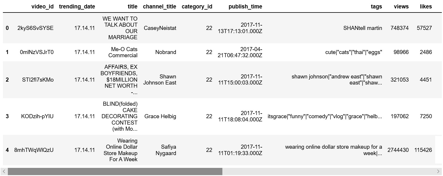
Figure 9.43: YouTube video data with category information
To get the video data with category information, we reused a lot of the code we developed in the previous exercises. It's important to write reusable and modular code so that we can simply use it without writing code from scratch.
- Calculate the likes-dislikes ratio for each category by adding the following code snippet in the next cell of the Jupyter Notebook:
# aggregate likes and dislikes by category
df_agg = df_join[['category', 'likes', 'dislikes']].groupby('category').sum()
# calculate ratio
df_agg['ratio_likes_dislikes'] = df_agg['likes'] /
df_agg['dislikes']
df_agg.head()
You should get the following output:

Figure 9.44: Ratio of likes to dislikes for each category
When we perform a groupby operation, it requires an aggregation action for each group. In this case, our aggregation action is sum. We are summing the likes and dislikes for each category.
In the pandas API, df_agg['likes'] / df_agg['dislikes'] returns a pandas series, each entry of which is the likes-dislikes ratio for each category. We assign the returned pandas series to the df_agg DataFrame's new column, ['rato_likes_dislikes'].
- Create a ratio_dag.py DAG script and add the following code to the script:
ratio_dag.py
1 import json
2 import os
3 import shutil
4 import sys
5 from datetime import datetime
6
7 import pandas as pd
8 from airflow import DAG
9 from airflow.operators.python_operator import PythonOperator
10
11
12 def filter_data(**kwargs):
13 # read data
14 path_vids = kwargs['dag_run'].conf['path_vids']
15 date = str(kwargs['dag_run'].conf['date'])
16
17 print(os.getcwd())
18 print(path_vids)
19
20 df_vids = pd.read_csv(path_vids, compression='zip')
21 .query('trending_date==@date')
22 # cache
23 try:
24 df_vids.to_csv('./tmp/data_vids.csv', index=False)
25 except FileNotFoundError:
26 os.mkdir('./tmp')
27 df_vids.to_csv('./tmp/data_vids.csv', index=False)
The full code is available at https://packt.live/2C8bqyP.
At a glance, you will notice that this DAG script is almost the same as the top_cat_dag.py DAG script from Exercise 9.06, Creating a DAG for Our Data Pipeline Using Airflow, except that there is one more operator and its corresponding Python callable, as shown in the following code:
def calc_ratio(**kwargs):
try:
df_join = pd.read_csv('./tmp/data_joined.csv')
except Exception as e:
print('>>>>>>>>>>>> Error: {}'.format(e))
sys.exit(1)
# aggreate likes and dislikes by category
df_agg = df_join[['category', 'likes', 'dislikes']].groupby('category').sum()
# calculate ratio
df_agg['ratio_likes_dislikes'] = df_agg['likes'] / df_agg['dislikes']
df_agg.reset_index('category')
.to_csv('./tmp/data_ratio.csv',
index=False)
op4 = PythonOperator(
task_id='calc_ratio',
python_callable=calc_ratio,
dag=dag)
This is the advantage of writing reusable and modular code. You can reuse most of the functions from previous exercises. Taking advantage of what you have already built is a very common practice in software engineering. One of the most often spoken phrases in the industry is, "Don't reinvent the wheel."
- Register the DAG by copying the ratio_dag.py DAG file to the Airflow home directory by running the following command in your Terminal:
cp ./ratio_dag.py ~/airflow/dags/
Note:
The Airflow webserver and scheduler should be stopped when you copy the DAG script to ~/airflow. We can stop them using Ctrl + C in the Command Prompt for Windows/Linux or Cmd + C for macOS. After the DAG script has been moved to the Airflow home directory, ~/airflow, we can launch the Airflow scheduler and webserver again. When the Airflow scheduler is launched again, it will register new DAGs from the DAG scripts in its home directory, ~/airflow. So, when we issue the airflow list_dags command, we can see new DAGs that are newly added.
- Verify whether the ratio_dag.py DAG is successfully registered in the Airflow system by running the following command:
airflow list_dags
You should get the following output:

Figure 9.45: List of DAGs registered in the Airflow system
The fourth entry from the bottom is our ratio_dag DAG. If your DAG is registered, you will see your DAG in the list returned by the airflow list_dags command.
- Launch the Airflow scheduler by running the following command in your Terminal:
airflow scheduler
You should get the following output:

Figure 9.46: Logs of the Airflow scheduler running in the foreground
Note
Launch the Airflow scheduler in the Activity09.01 directory. We are assuming that Activity09.01 is the working directory for the Airflow system.
When you launch an Airflow scheduler and it throws an error that reads attempt to write a readonly database, it means the user who launched the Airflow scheduler does not have write permission to the Airflow SQLite database file, airflow.db. One way to resolve the permission issue is to issue sudo chmod 644 ~/airflow/airflow.db in your Terminal and restart the Airflow scheduler so that the Airflow scheduler has write access to the database file.
- Trigger the DAG by running the following command:
airflow trigger_dag -c '
{
"path_vids": "../Data/USvideos.csv.zip",
"path_cats": "../Data/US_category_id.json",
"date": "17.14.11",
"path_output": "../Data/Ratio_Likes_Dislikes.csv"
}' 'ratio_dag'
You should get the following output:

Figure 9.47: ratio_dag is successfully scheduled to be executed
The trigger_dag action will trigger the DAG to run immediately. The CLI requires the DAG ID, ratio_dag. However, there is also a -c positional argument, which is used for passing parameters into each operator in our DAG.
- Launch the Airflow UI to monitor our DAG using the following command in a new Terminal:
airflow webserver
- Open your browser and go to http://localhost:8080/admin/ to open the UI of the Airflow system. Look for the ratio_dag DAG and click the Graph View icon as shown in the following figure:

Figure 9.48: Airflow UI dashboard
- Clicking the Graph View icon will redirect you to the following page:
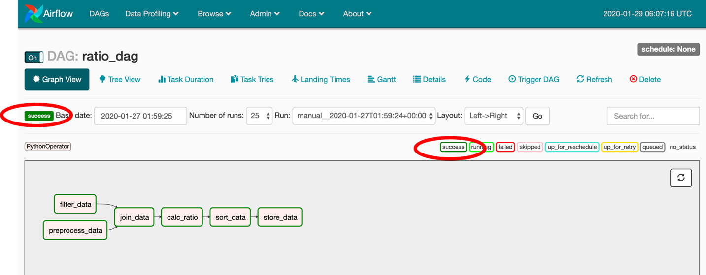
Figure 9.49: Monitoring a running pipeline
As we can see from this dashboard, every step in the pipeline is marked with a dark green border, which means the step completed successfully. All tiles have a dark green border, which means our data pipeline successfully finished.
- List the files in ../Data/ by running the following command in the Terminal:
ls ../Data/
You should get the following output:
Ratio_Likes_Dislikes.csv US_category_id.json USvideos.csv.zip top_10_trendy_cats.csv top_10_trendy_vids.csv
If you see the first file as Ratio_Likes_Dislikes.csv, it means the pipeline is successfully running.
- Open a new Python 3 Jupyter Notebook, import pandas, and use the read_csv function to read the Ratio_Likes_Dislikes.csv file, as shown in the following code:
import pandas as pd
pd.read_csv('../Data/Ratio_Likes_Dislikes.csv ')
You should get the following output:
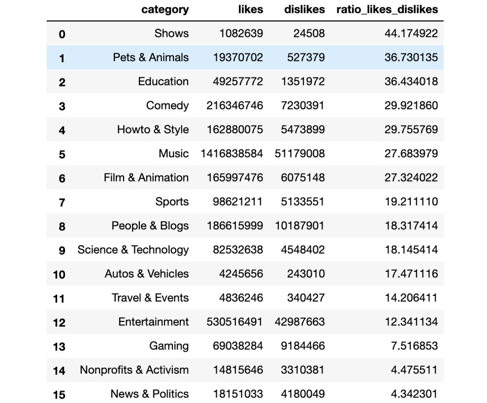
Figure 9.50: Ratio of likes to dislikes for each category
Note
To access the source code for this specific section, please refer to https://packt.live/32puIdZ.
10. Introduction to Data Storage on Cloud Services (AWS)
Activity 10.01: Transforming a Table Schema into Document Format and Uploading It to Cloud Storage
Solution
- Create a directory called Activity10.01 in the Chapter10 directory to store the files for this activity.
- Open your Terminal (macOS or Linux) or Command Prompt (Windows), navigate to the Chapter10 directory, and type in jupyter notebook.
- In the Jupyter Notebook, click the Activity10.01 directory, create a notebook file with a Python 3 kernel, and add the following code:
import os
import json
import boto3
import shutil
import pandas as pd
# set your bucket name here
# 'ch10-data' is NOT your bucket. It's just an example here
# you should replace your bucket below
BUCKET_NAME = 'ch10-data'
# 1. download data from S3 bucket
s3_resource = boto3.resource('s3')
try:
s3_resource.Bucket(BUCKET_NAME).download_file(
'New_York_City_Leading_Causes_of_Death.csv',
'./tmp/New_York_City_Leading_Causes_of_Death.csv')
except FileNotFoundError:
os.mkdir('tmp/')
s3_resource.Bucket(BUCKET_NAME).download_file(
'New_York_City_Leading_Causes_of_Death.csv',
'./tmp/New_York_City_Leading_Causes_of_Death.csv')
# read data
df_data = pd.read_csv('tmp/New_York_City_Leading_Causes_of_Death.csv')
df_data.head()
You should get the following output:

Figure 10.43: View of the New_York_City_Leading_Causes_of_Death.csv file
We downloaded a file from the S3 bucket first. Once the data was downloaded into the local directory, we used pandas to read the New_York_City_Leading_Causes_of_Death.csv file. Based on your first impression of the data, you can see that the data needs some preprocessing. For example, the value at row five of the Deaths column is ., whose data type is different compared to the rest of the values in the same column. There are two approaches we can use: we can either replace . with 0 or remove the row containing the . value.
- Preprocess the data using the following code:
# 2. replace "." with value 0 & and convert to float type
df_data_cleaned = df_data.replace('.', 0).astype({
'Deaths': float})
# check dtypes
df_data_cleaned.dtypes
You should get the following output:

Figure 10.44: Data type of each column
- Iterate over the different race-ethnicities and aggregate the death counts for each death that was caused, as shown in the following code:
# 3. get top 3 death causes for each ethnicity
top_causes = {}
for ethnicity, df_g in df_data_cleaned.groupby([
'Race Ethnicity']):
df_top_3_causes = df_g.groupby('Leading Cause')[['Deaths']].sum().sort_values(
'Deaths', ascending=False).head(3)
top_3_causes = df_top_3_causes.index.values.tolist()
top_causes.update({ethnicity: top_3_causes})
top_causes
You should get the following output:

Figure 10.45: Output of group by aggregate
We group the death count based on each death cause per ethnicity. Then, we sort death causes based on their death counts and keep the top three death causes for each ethnicity.
Note
The groupby clause in pandas can be hard to comprehend if this is your first time using pandas. It might be useful if you print the output of the data when you use the groupby clause so that you can understand what groupby is doing.
- As we can see, the last piece of output is a dictionary object. We need to dump this data into JSON format and write it to a JSON file using the following code:
with open('tmp/top_causes_per_ethnicity.json', 'w') as fout:
json.dump(top_causes, fout)
- The last step in this Extract, Transform, and Load (ETL) pipeline is to upload this output JSON file to the S3 bucket and remove the tmp/ directory, as shown in the following code:
# 5. upload data to S3
s3_resource.Bucket('ch10-data').upload_file(
'tmp/top_causes_per_ethnicity.json',
'top_causes_per_ethnicity.json')
# clean up tmp
shutil.rmtree('./tmp')
- Create a Python script named ETL_pipeline.py in the Activity10.01 directory and put all of the code snippets together in the Python script file. The file should contain the following code:
ETL_pipeline.py
14 # 1. download data from S3 bucket
15 s3_resource = boto3.resource('s3')
16 try:
17 s3_resource.Bucket(BUCKET_NAME).download_file(
18 'New_York_City_Leading_Causes_of_Death.csv',
19 './tmp/New_York_City_Leading_Causes_of_Death.csv')
20 except FileNotFoundError:
21 os.mkdir('tmp/')
22 s3_resource.Bucket(BUCKET_NAME).download_file(
23 'New_York_City_Leading_Causes_of_Death.csv',
24 './tmp/New_York_City_Leading_Causes_of_Death.csv')
The full code is available at https://packt.live/2Wh3e6q.
- Create a Python script named ETL_pipeline.py in the Activity10.01 directory. Add the preceding code snippet inside this Python script and save it.
- To run this pipeline, we will run the following command in a Terminal:
python ETL_pipeline.py
The script will create a top_causes_per_ethnicity.json file and upload it to the cloud.
- After the program has finished executing, we can verify whether the new data has been generated successfully or not by running the AWS CLI:
aws s3 ls s3://${BUCKET_NAME}/
You should get the following output:

Figure 10.46: Final output data has been successfully uploaded to the S3 bucket
Note
To access the source code for this specific section, please refer to https://packt.live/38TFoCt.
11. Building an Artificial Intelligence Algorithm
Activity 11.01: Implementing a Double Deep Q-Learning Algorithm to Solve the Cart Pole Problem
Solution
- In the Chapter11 directory, launch a Jupyter Notebook in your Terminal (macOS or Linux) or Command Prompt window (Windows).
- After the Jupyter Notebook is launched, create a new directory named Activity11.01. Inside the Activity11.01 directory, create a Python 3 notebook.
- Inside the Python 3 notebook, import all necessary modules and seed the environment as shown in the following code:
# import module
import random
import numpy as np
from itertools import count
from collections import deque
import torch
import torch.nn as nn
import torch.nn.functional as F
import torch.optim as optim
import gym
# make game
env = gym.make('CartPole-v1')
# seed the experiment
env.seed(9)
np.random.seed(9)
random.seed(9)
torch.manual_seed(9)
- Let's define our DQN as shown in the following code:
# define our policy
class DQN(nn.Module):
def __init__(self, observation_space, action_space):
super(DQN, self).__init__()
self.observation_space = observation_space
self.action_space = action_space
self.fc1 = nn.Linear(self.observation_space, 32)
self.fc2 = nn.Linear(32, 16)
self.fc3 = nn.Linear(16, self.action_space)
def forward(self, x):
x = F.relu(self.fc1(x))
x = F.relu(self.fc2(x))
x = self.fc3(x)
return x
We will use the three-layer feedforward neural network model from Exercise 11.04, Implementing a Deep Q-Learning Algorithm in PyTorch to Solve the Classic Cart Pole Problem.
- Next, we will create the agent to play the game as shown in the following code:
act01-notebook.ipynb
# define our agent
class Agent:
def __init__(self, policy_net, target_net):
MEMORY_SIZE = 10000
GAMMA = 0.6
BATCH_SIZE = 128
EXPLORATION_MAX = 0.9
EXPLORATION_MIN = 0.05
EXPLORATION_DECAY = 0.95
# 1, 2, 3
TARGET_UPDATE = 1
self.policy_net = policy_net
self.target_net = target_net
self.target_net.load_state_dict(policy_net.state_dict())
self.target_net.eval()
self.optimizer = optim.RMSprop(
policy_net.parameters(), lr=1e-3)
self.memory = deque(maxlen=MEMORY_SIZE)
self.gamma = GAMMA
self.batch_size = BATCH_SIZE
self.exploration_rate = EXPLORATION_MAX
self.exploration_min = EXPLORATION_MIN
self.exploration_decay = EXPLORATION_DECAY
self.target_update = TARGET_UPDATE
The full code is available at https://packt.live/309071q.
Notice that we implement one more method: update_target_net(). This method is for updating the weights for the parameters in the target network. During the training time, we keep the weights in the target network frozen for a while to add stability to the expected Q value. We only update the weights for the target network every once in a while. How often we update the weights for the target network is controlled using the TARGET_UPDATE parameter. TARGET_UPDATE = 1 means we update the weights for the target network after every 1 episode.
In the experience_replay() method, we train our policy network for every timestep. Recall the following loss function:

Figure 11.34: Loss function of the Q-learning algorithm
We use a policy network to calculate the Q values (the first term in the equation) for every previous state and chosen action. We then use the target network to calculate the expected Q values (the second term in the previous equation) using the next state, and the optimal action for every timestep.
- Finally, we will implement the double deep Q-learning training loop as shown in the following code:
act01-notebook.ipynb
# create policy
observation_space = env.observation_space.shape[0]
action_space = env.action_space.n
policy_net = DQN(observation_space, action_space)
target_net = DQN(observation_space, action_space)
# create agent
agent = Agent(policy_net, target_net)
# play game
game_durations = []
for i_episode in count(1):
state = env.reset()
state = torch.tensor([state]).float()
print("[ episode {} ] state={}".format(i_episode, state))
for t in range(1, 10000):
action = agent.select_action(state)
state_next, reward, done, _ = env.step(action.item())
if done:
state_next = None
The full code is available at https://packt.live/309071q.
Notice that we created two deep Q neural network instances, policy_net and target_net, using the same model architecture with the DQN class to successfully create the double deep-Q learning algorithm.
After you run the training loop, you should get the following output:

Figure 11.35: Output logs of the main training loop
Note
We will have loads of output data with 133 episode results. We have only shown the last section of it in the preceding figure.
- Lastly, let's visualize how our double deep Q-learning algorithm improves over time by running the following code:
import matplotlib.pyplot as plt
plt.style.use('ggplot')
plt.scatter(range(i_episode), game_durations)
plt.title('Game Duration Over Time')
plt.xlabel('game episode')
plt.ylabel('game duration')
plt.tight_layout()
You should get the following output:
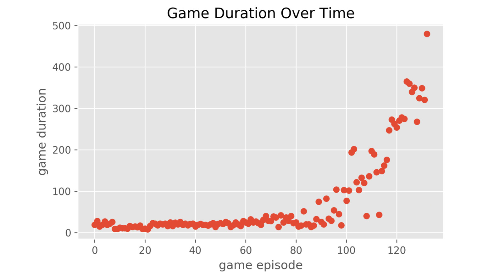
Figure 11.36: Game duration increases to 500 after 133 episodes
With the double Q-learning algorithm, the algorithm can converge faster in a more consistent fashion.
Note
To access the source code for this specific section, please refer to https://packt.live/309071q.
12. Productionizing Your AI Applications
Activity 12.01: Predicting the Class of a Passenger on the Titanic
Solution
- Create the Activity12.01 directory in the Chapter12 directory to store the files for this activity. Make sure that the Datasets directory contains the Titanic dataset subdirectory with two files in it: train.csv and test.csv.
- Start Jupyter Notebook and create a new Python 3 notebook in the Activity12.01 directory. Give the notebook the name development.
- Let's start by installing the pandas and sklearn Python libraries for model building. Enter the following code in the first cell:
!pip install pandas
!pip install sklearn
It should give the following output:

Figure 12.42: Installing pandas and sklearn
It will download the libraries and install them within your active Anaconda environment. There is a good chance that both frameworks are already available in your system, as part of Anaconda or from previous installations. If they are already installed, you will have the following output:

Figure 12.43: pandas and sklearn already installed
- Next, we import the pickle, pandas, and sklearn libraries:
import pickle
import pandas as pd
from sklearn.linear_model import LogisticRegression
- Load the training data into a pandas DataFrame object called train with the following statement:
# load the datasets
train = pd.read_csv('../../Datasets/Titanic/train.csv')
- After loading the training dataset, load the testing dataset with the following command:
test = pd.read_csv('../../Datasets/Titanic/test.csv')
- We'll now continue to prepare and clean the training dataset as mentioned in Chapter 3, Data Preparation. Machine learning models work best with numerical datatypes for all columns, so let's convert the Sex column to zeros and ones:
train.Sex = train.Sex.map({'male':0, 'female':1})
We have now transformed the values in the Sex column to either 0 (for male) or 1 (for female).
- Create the training set, X, which doesn't contain the Pclass output column, using the following code:
y = train.Pclass.copy()
X = train.drop(['Pclass'], axis=1)
Since the Pclass column contains our output value on which we have to train our model (the target values), we have to extract that from the dataset. We create a new dataset for it called y and then remove the column from the training dataset. We call the new training set X.
Now, let's do some feature engineering. We can be quite certain that a lot of the columns will not hold any predictive value as to whether a person survived. For example, the name of someone and their passenger ID are interchangeable and will not contribute much to the predictive power of the machine learning model.
- Remove the following set of columns that are not needed to predict the surviving passengers:
X.drop(['Name'], axis=1, inplace=True)
X.drop(['Embarked'], axis=1, inplace=True)
X.drop(['PassengerId'], axis=1, inplace=True)
X.drop(['Cabin'], axis=1, inplace=True)
X.drop(['Ticket'], axis=1, inplace=True)
# X.drop(['Fare'], axis=1, inplace=True)
- Replace the empty values with the mean age of all the passengers in the dataset:
X.Age.fillna(X.Age.mean(), inplace=True)
X.info()
- Let's now train the actual model. We'll create a logistic regression model, which is essentially a mathematical algorithm to separate the survivors from the people who died in the accident:
# create and train a simple model
from sklearn.linear_model import LogisticRegression
model = LogisticRegression()
model.fit(X, y)
- To see what the accuracy of the model is, we can run the full set of test data into the model and see in how many cases the algorithm produced a correct outcome using the following code:
# evaluate the model
model.score(X, y)
- Finally, we have to serialize (export) the model to a file with the pickle framework:
# export the model to pickle file
file = open('model.pkl', 'wb') # write in bytes
pickle.dump(model, file)
file.close()
The pickle.dump method serializes the model to a model.pkl file in the activity directory. The file has been opened as wb, which means that it will write bytes to disk. You can check the file exists in the Activity12.01 folder.
The second part of this activity is to load the model from disk in an API and expose the API.
- Create a new Python 3 notebook in the Activity12.01 directory and give it the name production.
Note
The production.ipynb file can be found here: https://packt.live/2ZqDc2n.
- In the first cell, enter the following line to install Flask:
!pip install flask
You'll get the following output:

Figure 12.44: Installing flask
If Flask is already installed, you will have the following output:

Figure 12.45: Flask already installed
- Now import the required libraries to deserialize the model and to create an API:
from flask import Flask, jsonify, request
import pickle
- The model that we trained in the first part was stored in the model.pkl file. Let's get that file from disk and deserialize the model into memory:
# load the model from pickle file
file = open('model.pkl', 'rb') # read bytes
model = pickle.load(file)
file.close()
We now have the same model running in our production environment (the production Jupyter Notebook) as in our model training environment (the development notebook from part 1 of this activity). To test the model, we can make a few predictions.
- Call the predict function of the model and give it an array of values that represent a person; the values are in the same order as the columns of the training set, as shown in the following code:
# get predictions from the model
print(model.predict([[1,0,36,2,0,14.67]]))
print(model.predict([[0,1,42,1,1,96.61]]))
- Let's continue with productionizing our model. We first must set up a Flask app, which we'll call ClassPredictor:
# create an API with Flask
app = Flask('ClassPredictor')
- The app is now an empty API with no HTTP endpoint exposed. To make things a bit more interesting and test whether it works, add a GET method that returns a simple string:
# call this: curl -X GET http://127.0.0.1:5000/foo
@app.route('/hi', methods=['GET'])
def bar():
result = 'hello!'
return result
- We have to add a new method to the API that executes the model and returns the result, as shown in the following code:
@app.route('/class', methods=['POST'])
def predict_class():
payload = request.get_json()
person = [payload['Survived'], payload['Sex'],
payload['Age'], payload['SibSb'],
payload['Parch'], payload['Fare']]
result = model.predict([person])
print(f'{person} -> {str(result)}')
return f'I predict that person {person} was in
class {result} of the Titanic '
app.run()
These lines define an HTTP POST method under the URL '/class'. When called, a person object is generated from the JSON payload. The person object, which is an array of input parameters for the model, is then passed to the model in the predict statement that we've seen before. The result is finally wrapped up in a string and returned to the caller.
Run the app again in the production Jupyter Notebook by executing the cell with the app.run() statement (stop it by clicking on the interrupt icon (
 ) or by typing Ctrl + C first, if needed). This time, we will test the API with a curl statement. cURL is a program that allows you to make an HTTP request across a network in a similar way to how a web browser makes requests, only the result will be just text instead of a graphical interface.
 - Open a new Terminal window or Anaconda prompt, and enter the following command:
curl -X POST -H "Content-Type: application/json" -d '{"Survived": 1, "Sex": 0, "Age": 72, "SibSb": 2, "Parch": 0, "Fare": 28.35}' http://127.0.0.1:5000/class
Note
There is a Jupyter Notebook called validation in GitHub that contains the same command in a cell. It can be found here: https://packt.live/3erHRp4
The string after the -d parameter in the curl script contains a JSON object with passenger data. The fields for a person have to be named explicitly.
After running this, you'll see the result of your API call that executed the model as follows in your Terminal or Anaconda prompt:
I predict that person [1, 0, 72, 2, 0,28.35] was in class [2] of the Titanic
Note
To access the source code for this specific section, please refer to https://packt.live/38T32iF.
Activity 12.02: Deploying a Machine Learning Model to a Kubernetes Cluster to Predict the Class of Titanic Passengers
Solution
- Create a new directory, Activity12.02, in the Chapter12 directory to store the files for this activity.
- Copy the model.pkl file from the Chapter12/Activity12.01 directory into the Activity12.02 directory.
- Let's create a new API first. Since we'll work outside of Jupyter on this one, we have to make sure that it runs on our local machine. Create a new file in the Activity12.02 folder called api.py. Open it with a text editor or an IDE and enter the following Python code:
from flask import Flask, request
import pickle
# load the model from pickle file
file = open('model.pkl', 'rb') # read bytes
model = pickle.load(file)
file.close()
# create an API with Flask
app = Flask('Titanic')
@app.route('/class', methods=['POST'])
def predict_class():
payload = request.get_json()
person = [payload['Survived'], payload['Sex'], payload['Age'], payload['SibSb'], payload['Parch'], payload['Fare']]
result = model.predict([person])
print(f'{person} -> {str(result)}')
return f'I predict that person {person} was in passenger class {result} of the Titanic '
app.run()
- Open a new Terminal or Anaconda Prompt and navigate to the Activity12.02 folder using the cd command. Enter the following command to check whether the API is working:
python api.py
If all is OK, you should get the message that your API is running on localhost.
- Test the local API by opening a new Terminal or Anaconda Prompt and enter the following code:
curl -X POST -H "Content-Type: application/json" -d '{"Survived": 0, "Sex": 1, "Age": 52, "SibSb": 1, "Parch": 0, "Fare": 82.35}' http://127.0.0.1:5000/class
- Add a new file in the Activity12.02 folder with the name requirements.txt. If we will deploy the API to another environment, it's good practice to indicate which libraries were used. To do so, Python offers the requirements.txt file, where you can write the dependencies of an application.
- Open the requirements.txt file in an editor and enter the following lines:
Flask
sklearn
pandas
Note
It's possible to specify the exact version, for example, by entering Flask==1.1.1. To see which version you have in your development environment, enter pip freeze. To export the current list of dependencies and store them as requirements.txt, enter pip freeze > requirements.txt.
Now, let's continue with containerizing the API to make it ready to deploy to a production environment. We need to create a Docker image, which is a template for creating the actual Docker containers that will be deployed.
- First, let's verify that Docker is installed correctly on your system. If you have followed the installation instructions, enter the following command in a Terminal or Anaconda Prompt:
sudo docker run hello-world
- Instead of working with a pre-defined Docker image, we want to set up our own. Docker images that are defined in strict files are named Dockerfile. So, let's add a new text file in the same directory and call it Dockerfile (without an extension). Open Dockerfile in a text editor or IDE, enter the following code and save the file:
FROM python:3.7
RUN mkdir /api
WORKDIR /api
ADD . /api/
RUN pip install -r ./requirements.txt
EXPOSE 5000
ENV PYTHONPATH="$PYTHONPATH:/api"
CMD ["python", "/api/api.py"]
- Open a new Terminal window (or Anaconda Prompt) in the Activity12.02 directory and enter the following command to create an image:
sudo docker build -t titanic .
In the output, it becomes clear that all steps in our Dockerfile have been followed. The Flask library is loaded, port 5000 is exposed, and the API is running.
- Let's check our local image repository again:
sudo docker image ls
It's great that we have a Docker image now, but that image has to be published to a Docker registry when we want to deploy it. Docker Hub is the central repository, but we don't want our Titanic API to end up there.
- Create a local registry and publish our image there, ready to be deployed to Kubernetes in the next part of this activity. Enter the following command in your Terminal:
docker run -d -p 6000:5000 --restart=always --name registry registry:2
This will download the registry libraries and will run a local registry. The output is as follows:

Figure 12.46: Creating a local registry
- Tag your Docker image with the following command to give it a suitable name:
docker tag titanic localhost:6000/titanic
- Now, push the titanic image to the running local registry with the following command:
docker push localhost:6000/titanic
This generates the following output:
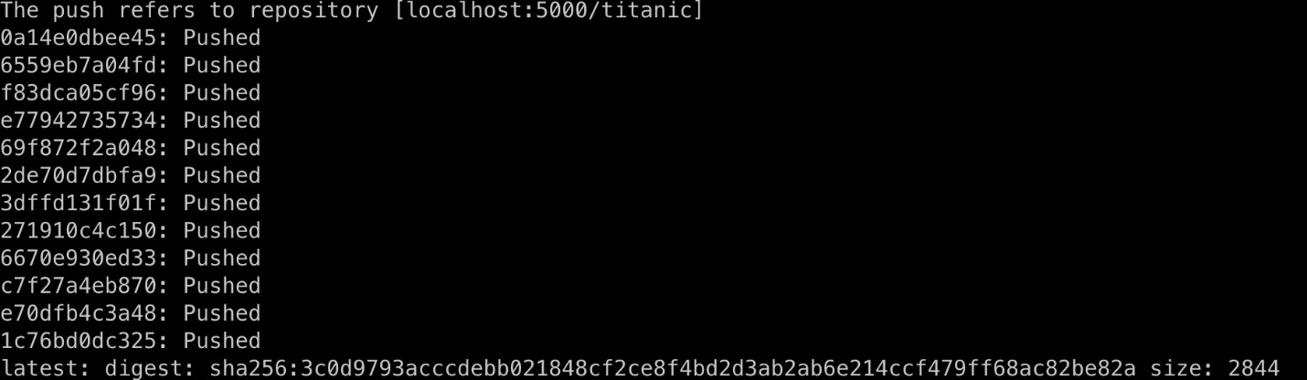
Figure 12.47: Pushing a Docker image to a local registry
- To verify that your image is pushed to the local registry, enter the following command:
curl -X GET http://localhost:6000/v2/titanic/tags/list
If all is well, you'll see the image with the latest tag:
{"name":"titanic","tags":["latest"]}
We have just successfully published our titanic image to that registry.
In the second part of this activity, we'll use the Docker image to host a container on a Kubernetes cluster.
- We first have to make sure that Minikube, the local version of Kubernetes, is running. Minikube is, in fact, a local virtual machine. Type the following command in a new Terminal or Anaconda Prompt:
minikube version
If all is OK, this will produce an output like minikube version: v1.8.1, along with a commit hashtag as follows:
minikube version: v1.8.1
commit: cbda04cf6bbe65e987ae52bb393c10099ab62014
- Start minikube by entering the following command in a new Terminal window or Anaconda Prompt:
minikube start --insecure-registry="localhost:6000"
If you're running within a virtual machine like VirtualBox, the command will be minikube start --driver=none. If all goes well, you'll get the following output:
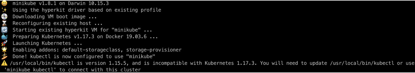
Figure 12.48: Starting Minikube
- Confirm that Minikube is running by using the following command:
minikube status
You'll get a status update like the following:
host: Running
kubelet: Running
apiserver: Running
kubeconfig: Configured
- If you want to look even further into your Kubernetes cluster, start up a dashboard with the following command:
minikube dashboard
This will open a browser window with a lot of useful information and configuration options:

Figure 12.49: The Kubernetes dashboard
- We have to connect our now-running Minikube Kubernetes cluster to a command-line interface, called kubectl. Type in the following command in your Terminal or Anaconda Prompt, as was already suggested in the previous output:
minikube kubectl
This will produce an output like the following:

Figure 12.50: Connecting Minikube to your kubectl command
You can read the kubectl controls the Kubernetes cluster manager line, which indicates that we can now use the kubectl tool to give commands to our cluster. You can get more information about the cluster with the kubectl version and kubectl get nodes commands:

Figure 12.51: Getting information from Minikube
- We have already created a Docker image and practiced deploying that to a Docker registry in part 1 of this activity. We'll rebuild the image now, but with the Docker daemon (process) of the Kubernetes cluster to make sure it lands on the Minikube cluster. Start by entering the following command:
eval $(minikube docker-env)
This command points our Terminal to use a different docker command, namely, the one in the Minikube environment.
- Let's build the container again but now with the Minikube. Enter the following command:
docker build -t titanic .
You'll get the same output as in part 1 of this activity.
- Create a Kubernetes deployment with the following command:
kubectl run titanic --image=titanic --image-pull-policy=Never
If this is successful, you'll see the following output:
deployment.apps/titanic created
- Verify the deployment of the container with the following command:
kubectl get deployments
This will produce a list of deployed containers:

Figure 12.52: Retrieving a list of deployed containers from Kubernetes
You can also check the Kubernetes dashboard, if you have started it, and check whether the deployment and Pod have been created:

Figure 12.53: The Kubernetes dashboard
- Now that our app is deployed, we want to connect to the titanic API. By default, the running containers can only be accessed by other resources (containers) in the same Kubernetes Pod. But we can instruct our cluster to create a network connection that allows communication from the outside world.:
kubectl port-forward titanic-6d8f58fc8b-znmx9 5000:5000
Note
In the preceding code, replace the name of the pod with your own; you can find it in the Kubernetes dashboard or by entering kubectl get pods
This will create a new port forwarding service in your Kubernetes cluster that forwards network traffic to the titanic Pod.
- To test the API, enter the following command in a new terminal window (while keeping the port forwarding running):
curl -X POST -H "Content-Type: application/json"
# -d '{"Survived": 1, "Sex": 0, "Age": 72, "SibSb": 2, "Parch": 0, "Fare": 68.35}' http://127.0.0.1:5000/class
This will produce the following output:
I predict that person [1, 0, 72, 2, 0, 68.35] was in passenger class [1] of the Titanic
Note
To access the source code for this specific section, please refer to https://packt.live/32s2PC3.
Activity 12.03: Predicting the Class of Titanic Passengers in Real Time
Solution
- In the Chapter12 directory, create the Activity12.03 directory to store the files for this activity.
- Open Jupyter Notebook and create a new Python 3 notebook called export_pmml in the Activity12.03 folder.
- Copy the model.pkl file from the Activity12.01 directory to the Activity12.03 directory. This can be done manually, or with the following statement in a notebook:
# copy the trained model for predicting the passenger
#class of a person
!cp ../Activity12.01/model.pkl .
- Enter the following line in the first cell of the new notebook:
!pip install sklearn2pmml
This will install the required library, which can export our models to the PMML format:

Figure 12.54: Installation of sklearn2pmml
If sklearn2pmml is already installed, you will have the following output:

Figure 12.55: sklearn2pmml already installed
- Create a new cell and enter the following lines to start using the pickle and sklearn2pmml libraries:
from sklearn2pmml import sklearn2pmml, make_pmml_pipeline
import pickle
- Deserialize the pickled model by executing the following code in a new cell:
# load the model from pickle file
file = open('model.pkl', 'rb') # read bytes
model = pickle.load(file)
file.close()
Now we can export the model to the PMML format.
- Enter the following lines in a new cell to create a pipeline, export the method, and write it to the PMML file:
pmml_pipeline = make_pmml_pipeline(model)
sklearn2pmml(pmml_pipeline, 'titanic_class.pmml')
- Check the contents of the generated titanic_class.pmml file by entering the following line in a new cell:
! cat titanic_class.pmml
This will produce the following output:
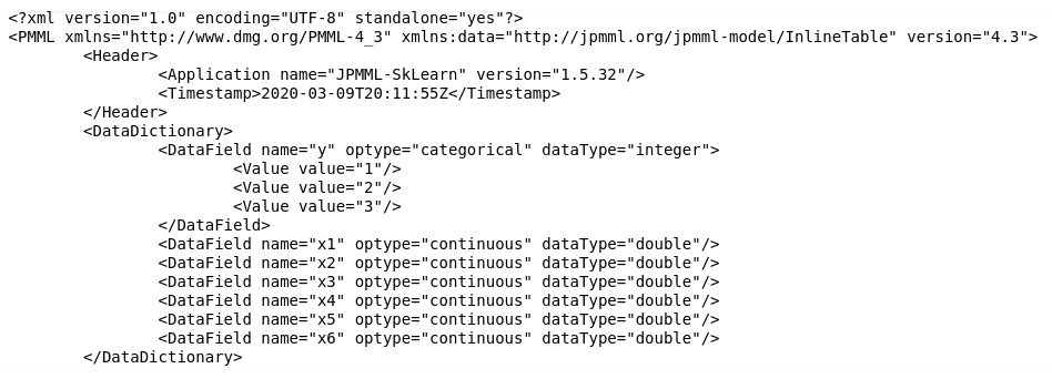
Figure 12.56: Viewing a PMML model in a Jupyter Notebook
Now let's create a streaming job. We'll use Apache Flink for this. We'll write the code with an example from IntelliJ IDEA. You can also choose another IDE. It's also possible (though not recommended) to use a plain text editor and run the code from a Terminal or command line.
- Open a new Terminal window in the Activity12.03 directory and enter the following lines to set up Apache Flink:
mvn archetype:generate
-DarchetypeGroupId=org.apache.flink
-DarchetypeArtifactId=flink-quickstart-java
-DarchetypeVersion=1.10.0
- During the installation, enter the following values:
groupId: com
artifactId: titanic_class
version: 0.0.1
package: packt
This will generate a project from a template.
- Open your favorite IDE (IntelliJ IDEA, Eclipse, or another) and import the generated files by selecting the pom.xml file.
- Remove the BatchJob.java file; we don't need it since we're only building a streaming job.
- Copy the titanic_class.pmml file that we created in Step 8 to the titanic_class/src/resources directory.
- If you installed JDK and Maven, you should be able to compile the code. Type the following in your Terminal to compile the code and package it into a JAR file:
mvn clean package
In the output, you'll see BUILD SUCCESS, which indicates that you now have a working Java program.
Let's start by testing the job – first, the Maven template generated code that can be deployed to a Flink cluster.
- Since we want to test locally first, let's change the configuration a bit. Open the pom.xml file and remove the <provided> tags in the dependencies of flink-java and flink-streaming-java; these tags are single lines within the <dependency> elements. The file will look like the following:
Figure 12.57: The pom.xml file with the provided tags removed for Flink dependencies
Save the file, then import the Maven changes.
- Open the StreamingJob.java file in your IDE and add the following lines at the top:
import
org.apache.flink.api.common.serialization.SimpleStringEncoder;
import org.apache.flink.core.fs.Path;
import org.apache.flink.streaming.api.datastream.DataStream;
import org.apache.flink.api.common.functions.MapFunction;
import
org.apache.flink.streaming.api.datastream.
SingleOutputStreamOperator;
import
org.apache.flink.streaming.api.environment.
StreamExecutionEnvironment;
import
org.apache.flink.streaming.api.functions.
sink.filesystem.StreamingFileSink;
These lines will add the necessary Flink libraries to our class file.
- In the middle part of the file, within the main function, add the following lines:
DataStream<String> dataStream = env.socketTextStream(
"localhost", 1234, " ");
StreamingFileSink<String> sink = StreamingFileSink
.forRowFormat(new Path("out"),
new SimpleStringEncoder<String>("UTF-8"))
.build();
dataStream.addSink(sink);
This code sets up a data stream that listens to a local socket on port 1234. It takes the lines and writes (sinks) the lines to a file in the out directory.
- To write to a local socket, we use the Netcat tool. Test the simple code by opening a Terminal and typing the following command:
nc -l -p 1234
You get a prompt to enter lines. Leave it open for now.
- Go back to your IDE and run the StreamingJob.main() method. Alternatively, type the following in a Terminal to build and run the code:
mvn clean package
mvn exec:java -Dexec.mainClass="packt.StreamingJob"
These lines are the Maven instructions to compile the code, package it into a JAR file, and run the file with an entry point in the packt.StreamingJob class that contains our main function.
- In the Terminal that's still running Netcat, type a few lines of text, followed by Enter for each line, as follows:

Figure 12.58: Running a Flink job that processes input from a local socket
- Now check the output in the out directory. You should see a subfolder with a date and time, and a file for each line that was entered in the input socket.
- We have to add JPMML dependencies to our project for this. Add the following lines to pom.xml and import the Maven changes:
<dependency>
<groupId>org.jpmml</groupId>
<artifactId>pmml-evaluator</artifactId>
<version>1.4.15</version>
</dependency>
<dependency>
<groupId>org.jpmml</groupId>
<artifactId>pmml-evaluator-extension</artifactId>
<version>1.4.15</version>
</dependency>
- Edit the StreamingJob.java file again and add the following lines at the top of the file:
import org.dmg.pmml.FieldName;
import org.jpmml.evaluator.*;
import org.jpmml.evaluator.visitors.DefaultVisitorBattery;
import java.io.File;
import java.util.LinkedHashMap;
import java.util.List;
import java.util.Map;
These lines import the required PMML and common Java libraries for working with PMML files.
- Enter the following lines at the beginning of the main method:
// load PMML Evaluator evaluator= getPmmlEvaluator("titanic_class.pmml");
// get input fields List<? Extends InputField> inputFields = evaluator.getInputFields();
This code deserializes the model from PMML, loading the model in memory ready to be executed. The list of input fields will come in handy in the next step.
We are now ready to parse incoming messages as persons that can be evaluated according to whether they survived the Titanic disaster. The input values will be in a comma-separated string with the values survived, sex, age, number of siblings on board, number of parents on board, and fare paid. For example, "1,1,19,0,2,77.15" indicates a woman of 19 years old who entered the ship with her two parents and paid 77.15 for the ticket.
- The PMML evaluator expects a map of FieldName value objects so we first have to convert the input strings. To do so, add the following lines to the class:
SingleOutputStreamOperator<String> mapped = dataStream.map(new MapFunction<String, String>() {
@Override
public String map(String s) throws Exception {
System.out.println("EVENT: " + s);
Map<FieldName, FieldValue> arguments = new LinkedHashMap<>();
String[] values = s.split(",");
// prepare model evaluation
for (int i = 0; i < values.length; i++) {
FieldName inputName = inputFields.get(i).getName();
FieldValue inputValue = inputFields.get(i).prepare(values[i]);
arguments.put(inputName, inputValue);
}
// execute the model
Map<FieldName, ?> results = evaluator.evaluate(arguments);
// Decoupling results from the JPMML-Evaluator runtime environment
Map<String, ?> resultRecord = EvaluatorUtil.decodeAll(results);
System.out.println(resultRecord);
return s;
}
});
This code adds a map method to the stream processing job that splits the input string and uses the resulting string values to build a set of arguments for the machine learning model.
- Now, if you run this code together with Netcat for the input socket, you can get real-time predictions from the model. Enter the following set of comma-separated values in the nc prompt that is already running, followed by Enter, and see what predictions are made:
1,1,13,1,56.91
0,0,81,0,0,120.96
1,0,41,1,1,18.11
You should get the following output:

Figure 12.59: Output of the Flink job that predicts the class of Titanic passengers
Note
To access the source code for this specific section, please refer to https://packt.live/38SssNr.