
In this chapter, we will explore the broad range of capabilities of AI and look at some of the fields that it is changing. We will cover four areas in which AI is used in detail: medicine, language translation, subtitle generation, and forecasting. Then we will dive into a text classification example where you will build your first AI system – a basic text classifier that can identify when a news headline is regarded as "clickbait." We will look at optimization – an important topic for most machine learning systems that need to operate on a large scale. Finally, we will examine different kinds of hardware, including memory, processes, and storage, and will also see how we can reduce costs when renting this hardware from a cloud vendor.
By the end of this chapter, you will understand what kind of tasks machine learning can be used to perform. You will be able to build your own basic machine learning systems, using a popular Python library, sklearn. You will also be able to optimize the hardware of large systems and reduce costs while storing your data in a logical way.
Introduction
Machine learning, which is a subset of Artificial Intelligence (AI), has had a major influence on nearly every field you can imagine and can solve a wide variety of problems and tasks. Do you want to detect cancer better? You can train an image classifier to inspect mammograms. Do you want to communicate with people in other languages? Machine translation will help you. From ambitious projects such as self-driving cars and astronomical discoveries to fixing minor annoyances such as email spam, machine learning has taken the world by storm, and those who understand what it can do and how to build machine learning systems will be at the forefront of human advancement.
At the heart of any machine learning project is data. Many people, on first coming across the concept of machine learning, assume that it is possible to take mounds of data, shove it into a machine, and have the machine autonomously learn. But it's not so simple. Instead, machines need meticulously structured, organized, and clean data, often in huge quantities. The more data there is, the more difficult it becomes to store, process, and analyze the data, and it is therefore vital to optimize data storage at all stages of storage and usage.
This is a problem. How can we build efficient machine learning systems that do not waste our time or resources?
This course will show you practical real-world examples of how to do exactly that. You will learn how to make your data work for you as efficiently as possible, often by example.
We assume that you are no novice at working with data and that you understand and have used various filesystems, file formats, databases, and storage solutions for digital data. In this book, we will focus specifically on data for machine learning and show how this differs from storing general-purpose data.
Machine learning comes in many different forms, but concepts from linear algebra are core to many of the most important machine learning algorithms. In classical computer science, the focus is often on data structures such as arrays, linked lists, hash tables, and trees. In machine learning, while these structures are still important, you will more often need to work with data in the form of vectors, matrices, and tensors.
Because of this focus on data structures from linear algebra, other components of storage solutions have nuances too. Some processors are optimized at the hardware level for vectorized operations. Some file formats handle this kind of data better too, and there are specialized data structures to store data in this form efficiently as well.
Problems Solved by Machine Learning
Before we get our hands too dirty with learning how to store and process machine learning data in efficient ways, let's take a step back. What kinds of real-world problems can we solve using machine learning?
Machine learning is not a new concept, but with new algorithms and better hardware, it has seen a resurgence over the last few years. This means it has received significant attention from many diverse fields. Although the applications of AI are almost uncountable, nearly all of these stem from a far smaller number of subfields within machine learning.
With that in mind, we'll start by examining one problem that machine learning can solve in each of the main subfields of image processing, text and language processing, audio processing, and time series analysis. Some problems, such as navigation systems, need to combine many of these fields, but the fundamental concepts remain very similar. We'll start by looking at image processing: we do not fully understand all the complexities behind how humans see, so helping computers 'see' is a particularly challenging task.
Image Processing – Detecting Cancer in Mammograms with Computer Vision
For classification tasks, the goal is to look at some data and decide which class it belongs to. In simple cases, there are only two classes: positive and negative. When a doctor looks at a mammogram to assess whether a patient has cancer, the doctor is looking for specific patterns and signs. The doctor then makes a diagnosis based on the patterns.
As a slight simplification, a doctor looks at a mammogram X-ray and classifies it into one of two classes: 'cancer' (positive) or 'healthy' (negative). Using image processing and machine learning, a computer can be trained to do the same thing. The computer is fed thousands or millions of X-rays in the form of digital images. Interpreting these as a set of matrices with associated labels, the computer uses a machine-learning algorithm to learn which patterns are indicative of cancer and which are not.
It's an emerging field, but a very promising-looking one. In January 2020, Google published a paper titled International evaluation of an AI system for breast cancer screening, which showed results that indicated their AI system was able to identify cancer in mammograms not only faster but also more reliably than human doctors.
Although images and language may seem very different, many techniques from image processing can be used to help machines better understand and learn human languages. Let's take a look at how AI has advanced the field of Natural Language Processing (NLP).
Text and Language Processing – Google Translate
While computers are great at repetitive mechanical tasks such as solving well-defined equations, and humans are better at more creative tasks such as drawing, it is likely that if computers and humans could work better together, their complementary skills would be more valuable than they are individually. How can we help machines and humans work better together? A desirable approach is to allow computers to act more like humans, fostering closer collaboration.
To this end, we have tried to make computers take on traditionally 'human' characteristics, such as the following:
- Look like us: In 2016, David Hanson created a human-like 'social' robot named Sophia, which, apart from having a transparent skull, looks like a human female, and is partially modeled on Audrey Hepburn:

Figure 1.1: Sophia – The first robot citizen at the AI for Good Global Summit 2018 (ITU pictures)
- Walk like us: Shortly after Sophia was shown to the world, Agility Robotics released 'Cassie' – a robot that looks far less human than Sophia but can walk on two legs in a very similar way to humans:

Figure 1.2: Cassie, a walking robot, photo by Oregon State University (CCSA)
- Play a wide variety of games: Computers can now beat even the best humans at rock, paper, scissors; chess; Go; and Super Mario Bros:

Figure 1.3: Rock, paper, scissors (OpenClipart-Vectors)
But making computers talk like us is hard, and making them understand us is still an unsolved problem and an area of active research.
That said, there is strong progress, especially in the field of machine translation, which is one form of language understanding. Machine translation algorithms can take a written text in one language and output the equivalent text in another language – for example, if you want to read a news article in French but you can only speak English, you can simply paste the article into Google Translate and it will spit out almost perfect English.
As with other machine learning systems, a vital ingredient for machine translation is a huge dataset. And hand-in-hand with a huge dataset, we need optimized data structures and storage methods to successfully create such a system. There are thousands of reasons why you might want to read a text in a language that you do not understand, from ordering at a foreign restaurant to studying old literature to conducting business with people in other countries.
A good example of machine translation in action is eBay, which improved its automatic translation capabilities in 2014. Imagine being a native Spanish speaker based in Latin America buying goods online from a native English speaker based in the US. You'd want to search for products in the language that you are most comfortable with, and you would want to read the details about the product, its condition, and shipping possibilities in Spanish too. Due to the large amount of eBay sales between Latin America and the USA, eBay tried to solve exactly this problem using AI. After improving its machine translation systems, eBay – as shown in the study "Does Machine Translation Affect International Trade? Evidence from a Large Digital Platform" – saw a 10.9 percent increase in purchases where the seller and buyer spoke different languages.
The translation of text is complicated, but at least writing is consistent. Spoken language can be even more complicated due to the complexities of sound waves, different accents, and different voice pitches: let's take a look at audio processing.
Audio Processing – Automatically Generated Subtitles
Subtitles on videos are very useful. They help deaf people access video content and also allow video content to be shared across language barriers. The problem with subtitles is that they are difficult to create. Traditionally, to create subtitles, a person with specialized knowledge had to watch an entire video, potentially multiple times, typing out every audible word. Then each word had to be carefully aligned to the correct timestamp in the video file. How could we create subtitles for every video on YouTube? Once again, AI can come to our aid.
Years ago, Google introduced YouTube videos with automatically generated captions, and these have steadily improved in quality. Being able to read what people are saying as they talk is useful for millions of hard of hearing people and billions of people listening to audio or video content in their second or third language.
Similarly, California State University has used automatic captions to make their content available for deaf people.
We have now seen how AI can help computers act more like humans, but AI can also help computers be more efficient at other tasks, such as mathematics and analysis, including time series analysis, which is used across many fields. Let's study it in the next section.
Time Series Analysis
Seeing how machines can help us with health, communication, and disabilities might already make AI seem almost magical, but another area where AI shines is predicting the future. A common method for forecasting is time series analysis, which involves studying historical data, looking for trends, and assuming that these will hold in the future as well.
In an arguably less noble pursuit than medical advances, one of the most popular applications for time series analysis is in financial trading. If we can predict the rise and fall of stock prices, then we can be rich (as long as we don't share our knowledge too widely).
Despite decades of research and many attempts, it is not completely clear whether machines can reliably turn data directly into money by trading on global stock markets. Nonetheless, billions and potentially trillions of dollars change hands automatically every day, powered by AI predicting which assets will be valuable in the future.
Optimizing the Storing and Processing of Data for Machine Learning Problems
All of the preceding uses for artificial intelligence rely heavily on optimized data storage and processing. Optimization is necessary for machine learning because the data size can be huge, as seen in the following examples:
- A single X-ray file can be many gigabytes in size.
- Translation corpora (large collections of texts) can reach billions of sentences.
- YouTube's stored data is measured in exabytes.
- Financial data might seem like just a few numbers; these are generated in such large quantities per second that the New York Stock Exchange generates 1 TB of data daily.
While every machine learning system is unique, in many systems, data touches the same components. In a hypothetical machine learning system, data might be dealt with as follows:

Figure 1.4: Hardware used in a hypothetical machine learning system
Each of these is a highly specialized piece of hardware, and although not all of them store data for long periods in the way traditional hard disks or tape backups do, it is important to know how data storage can be optimized at each stage. Let's dive into a text classification AI project to see how optimizations can be applied at some stages.
Diving into Text Classification
Let's take a look at a practical use for the machine learning theory described in the preceding section. If you have spent any time reading news articles online, you'll probably have noticed that many sites take advantage of so-called "clickbait" – the practice of publishing headlines that deliberately withhold crucial information and imply that something exceptional happened to make readers click on an otherwise fairly boring article.
For example, "17 Insanely Awesome Starbucks You Need To See" is an example of a real headline that we can call "clickbait." It uses several tricks to try to make readers click through to the full article, even though the article itself is not very interesting: it uses an exact number (17), invoking curiosity to find out what all 17 are; it uses exaggeration ("insanely"), although there is nothing actually "insane" about the Starbucks in question; and it claims that you "need" to see them, although you can probably do just fine without.
On the other hand, publications with stronger commitments to ethical journalism would publish a headline such as "Ralph Nader enters US presidential race as independent" (another real headline). This headline, in direct contrast to the other one, is not clickbait. It is stating a simple fact; it is giving as much relevant information as possible upfront, and it is not trying to mislead the reader in any way.
To a computer, these headlines are difficult to tell apart. They both use standard English words, they are both similar in length, and there are not any specific rules that let you say with certainty "this is how to identify that a headline can be classified as clickbait."
This is a great example to use for machine learning – we, as humans, can tell which headlines are clickbait and which are not, but it is difficult to express this distinction as specific rules. Therefore, it makes sense to show a machine thousands of labeled examples – telling it 'these are clickbait, and these are not' – and see whether the machine can infer the rules on its own.
There are some important fundamentals and terminologies you need to be familiar with to fully follow along. For convenience, we'll summarize these here, but if you are not familiar with vectorization, training data, labels, classification, and evaluation, please note that these are complicated topics and that you may need to spend some time reading more about these in third-party resources.
Let's start by taking a look at TF-IDF vectorization.
Looking at TF-IDF Vectorization
Humans are used to reading and writing text, but computers prefer working with numerical data. For machines to be able to meaningfully process natural language text, we need to first convert this text into a meaningful binary format. There are many different ways of doing this, but a simple one is TF-IDF or Term Frequency, Inverse Document Frequency.
The fundamental idea of TF-IDF is that the more often a word appears in a text, the more important that word is. So, in an article about "electric cars," it is likely that the words "electric" and "car" will appear often, indicating that these words should be given more attention in any analysis that we do. Unfortunately, there are many common words, such as "the," and even though these words appear frequently, they are not important. To compensate for this, we don't only look at term frequency, but also inverse document frequency. A word that often appears in a single article but does not appear in many different articles is more important than a term that appears often in all articles. The exact weighting equation is not too important, and our Python library, sklearn, will take care of it for us, but out of interest, instead of using simple frequency counts as in the previous example, we will use the following equation:
word_freq(w, d) x log (N/doc_freq(w))
Here:
- word_freq(w,d) means the count of word w in document d.
- N means the total number of documents in our collection.
- doc_freq(w) means the number of documents that the word w appears in.
The point of vectorization is to transform the text into vectors, or an array of numbers that can be processed by a machine.
Term frequency, the first part of TF-IDF, relates to how often specific words are used. We'll start by looking at a manual example of vectorization using only term frequency, and then see how we can use a standard Python library for the full version of TF-IDF.
Counter-intuitively, we can ignore the order that the words in a given text are presented in and look only at their frequency. For example, we have two very short sentences in two documents, shown as follows:
- "a cat and a dog"
- "a cat and a fish"
We could first create a mapping table, assigning a single number to each word across all of our documents. This would look as follows:
'a' = 0
'cat' = 1
'and' = 2
'dog' = 3 (We skip the second "a" in the first document, as we already assigned it to a number.)
'fish'= 4 (We skip all the words before fish in the second document as they are all already assigned a number.)
The numbers map to what can be used as indices in an array. We will create a single array, containing only numbers to represent our document. The zeroth element of the array will indicate how many times the word "a" appears, as this was assigned the index "0." Once we have this mapping, we can represent both documents entirely numerically with arrays, as shown in the following figure:

Figure 1.5: Vectorized example – values and indices
The 2 at the zeroth index of the first array indicates that the word a appears twice in our first document, and the next three ones indicate that the words cat, and, and dog appear once each. Fish doesn't appear at all in the first document, so the 4th index of the array is a 0. The second array looks very similar, but there is a 0 at the 3rd index to indicate that the dog doesn't appear and a 1 at the fourth index to indicate that fish appears once.
Note that the ordering is lost. The documents a cat dog and and a cat and a dog look the same now, but surprisingly this is hardly ever a problem in text processing.
We have seen how to convert text into a vectorized form for computers to read, which is an important first step. Before we get to use this in a practical example, we will define some basic terminology in machine learning classification tasks.
Looking at Terminology in Text Classification Tasks
In a classification problem, we have data and labels – in our case, the data is the collection of headlines (clickbait and non-clickbait) and the labels are the indication of whether a specific headline is in fact "clickbait" or is "not clickbait."
We also have the terms training and evaluation. In the first part of the project, we'll feed both the data and the labels into our machine learning algorithm and it will try to derive a function that maps the data to the labels. We evaluate our model using different metrics, but a common and simple one is accuracy, which is how often the machine can predict the correct label without having access to it.
We'll be using two supervised machine learning algorithms in our project:
- Support Vector Machine (SVM): SVMs project data into higher dimensional space and look for decision boundaries.
- Multi-layer perceptron (MLP): MLPs are in some ways similar to SVMs but are loosely inspired by human brains, and contain a network of "neurons" that can send signals to each other.
The latter is a form of neural network, the model that has become the poster-child of machine learning and artificial intelligence.
We'll also be using a specialized data structure called a sparse matrix. For matrices that contain many zeros, it is not efficient to store every zero. We can, therefore, use a specialized data structure that stores only the non-zero values, but that nonetheless behaves like a normal matrix in many scenarios. Sparse matrices can be many times smaller than dense or normal matrices.
In the next exercise, you'll load a dataset, vectorize it using TF-IDF, and train both an SVM and an MLP classifier using this dataset.
Exercise 1.01: Training a Machine Learning Model to Identify Clickbait Headlines
In this exercise, we'll build a simple clickbait classifier that will automatically classify headlines as "clickbait" or "normal." We won't have to write any rules to tell the algorithm how to do this, as it will learn from examples.
We'll use the Python sklearn library to show how to train a machine learning algorithm that can differentiate between the two classes of "clickbait" and "normal" headlines. Along the way, we'll compare different ways of storing data and show how choosing the correct data structures for storing data can have a large effect on the overall project's feasibility.
We will use a clickbait dataset that contains 10,000 headlines: 5,000 are examples of clickbait while the other 5,000 are normal headlines.
The dataset can be found in our GitHub repository at https://packt.live/2C72sBN
You need to download the clickbait-headlines.tsv file from the GitHub repository.
Before proceeding with the exercises, we need to set up a Python 3 environment with sklearn and Anaconda (for Jupyter Notebook) installed. Please follow the instructions in the Preface to install it.
Perform the following steps to complete the exercise:
- Create a directory, Chapter01, for all the exercises of this chapter. In the Chapter01 directory, create two directories named Datasets and Exercise01.01.
Note
If you are downloading the code bundle from https://packt.live/3fpBOmh, then the Dataset folder is present outside Chapter01 folder.
- Move the downloaded clickbait-headlines.tsv file to the Datasets directory.
- Open your Terminal (macOS or Linux) or Command Prompt (Windows), navigate to the Chapter01 directory, and type jupyter notebook. The Jupyter Notebook should look like the following screenshot:

Figure 1.6: The Chapter01 directory in Jupyter Notebook
- Create a new Jupyter Notebook. Read in the dataset file and check its size as shown in the following code:
import os
dataset_filename = "../../Datasets/clickbait-headlines.tsv"
print("File: {} Size: {} MBs"
.format(dataset_filename,
round(os.path.getsize(
dataset_filename)/1024/1024, 2)))
Note
Make sure you change the path of the TSV fie (highlighted) based on where you have saved it on your system. The code snippet shown here uses a backslash ( ) to split the logic across multiple lines. When the code is executed, Python will ignore the backslash, and treat the code on the next line as a direct continuation of the current line.
You should get the following output:
File: ../Datasets/clickbait-headlines.tsv
Size: 0.55 MBs
We first import the os library from Python, which is a standard library for running operating system-level commands. Further, we define the path to the dataset file as the dataset_filename variable. Lastly, we print out the size of the file using the os library and the getsize() function. We can see in the output that the file is less than 1 MB in size.
- Read the contents of the file from disk and split each line into data and label components, as shown in the following code:
import csv
data = []
labels = []
with open(dataset_filename, encoding="utf8") as f:
reader = csv.reader(f, delimiter=" ")
for line in reader:
try:
data.append(line[0])
labels.append(line[1])
except Exception as e:
print(e)
print(data[:3])
print(labels[:3])
You should get the following output:
["Egypt's top envoy in Iraq confirmed killed",
'Carter: Race relations in Palestine are worse than apartheid',
'After Years Of Dutiful Service, The Shiba Who Ran A Tobacco Shop Retires']
['0', '0', '1']
We import the csv Python library, which is useful for processing our file and is in the tab-separated values (TSV) file format. We then define two empty arrays, data, and labels. We open the file, create a CSV reader, and indicate what kind of delimiter (" ", or a tab character) is used. Then, loop through each line of the file and add the first element to the data array and the second element to the labels array. If anything goes wrong, we print out an error message to indicate this. Finally, we print out the first three elements of each of our arrays. They match up, so the first element in our data array is linked to the first element in our labels array. From the output, we see that the first two elements are 0 or "not clickbait," while the last element is identified as 1, indicating a clickbait headline.
- Create vectors from our text data using the sklearn library, while showing how long it takes, as shown in the following code:
%%time
from sklearn.feature_extraction.text import TfidfVectorizer
vectorizer = TfidfVectorizer()
vectors = vectorizer.fit_transform(data)
print("The dimensions of our vectors:")
print(vectors.shape)
print("- - -")
You should get the following output:
The dimensions of our vectors:
(10000, 13169)
- - -
Wall time: 294 ms
Note
Some outputs for this exercise may vary from the ones you see here.
The first line is a special Jupyter Notebook command saying that the code should output the total time taken. Then we import a TfidfVectorizer from the sklearn library. We initialize vectorizer and call the fit_transform() function, which assigns each word to an index and creates the resulting vectors from the text data in a single step. Finally, we print out the shape of the vectors, noticing that it is 10,000 rows (the number of headlines) by 13,169 columns (the number of unique words across all headlines). We can see from the timing output that it took a total of around 200 ms to run this code.
- Check how much memory our vectors are taking up in their sparse format compared to a dense format vector, as shown in the following code:
print("The data type of our vectors")
print(type(vectors))
print("- - -")
print("The size of our vectors (MB):")
print(vectors.data.nbytes/1024/1024)
print("- - -")
print("The size of our vectors in dense format (MB):")
print(vectors.todense().nbytes/1024/1024)
print("- - - ")
print("Number of non zero elements in our vectors")
print(vectors.nnz)
print("- - -")
You should get the following output:
The data type of our vectors
<class 'scipy.sparse.csr.csr_matrix'>
- - -
The size of our vectors (MB):
0.6759414672851562
- - -
The size of our vectors in dense format (MB):
1004.7149658203125
- - -
Number of non zero elements in our vectors
88597
- - -
We printed out the type of the vectors and saw that it was csr_matrix or a compressed sparse row matrix, which is the default data structure used by sklearn for vectors. In memory, it takes up only 0.68 MB of space. Next, we call the todense() function, which converts the data structure to a standard dense matrix. We check the size again and find the size is over 1 GB. Finally, we output the nnz (number of non-zero elements) and see that there were around 88,000 non-zero elements stored. Because we had 10,000 rows and 13,169 columns, the total number of elements is 131,690,000, which is why the dense matrix uses so much more memory.
- For machine learning, we need to split our data into a train portion for training and a test portion to evaluate how good our model is, using the following code:
from sklearn.model_selection import train_test_split
X_train, X_test,
y_train, y_test = train_test_split(vectors,
labels, test_size=0.2)
print(X_train.shape)
print(X_test.shape)
You should get the following output:
(8000, 13169)
(2000, 13169)
We imported the train_test_split function from sklearn and split our two arrays (vectors and labels) into four arrays (X_train, X_test, y_train, and y_test). The y prefix indicates labels and the X prefix indicates vectorized data. We use the test_size=0.2 argument to indicate that we want 20% of our data held back for testing. We then print out each shape to show that 80% (8,000) of the headlines are in the training set and that 20% (2,000) of the headlines are in the test set. Because each dataset was vectorized at the same time, each still has 13,169 dimensions or possible words.
- Initialize the SVC classifier, train it, and generate predictions with the following code:
%%time
from sklearn.svm import LinearSVC
svm_classifier = LinearSVC()
svm_classifier.fit(X_train, y_train)
predictions = svm_classifier.predict(X_test)
You should get the following output:
Wall time: 55 ms
Note
The preceding output will vary based on your system configuration.
We import the LinearSVC model from sklearn and initialize an instance of it. Then we give it the training data and training labels (note that it does not have access to the test data at this stage). Finally, we give it the testing data, but without the testing labels, and ask it to guess which of the headlines in the held-out test set are clickbait. We call these predictions. To get some insight into what is happening, let's take a look at some of these predictions and compare them to the real labels.
- Output the first 10 headlines along with their predicted class and true class by running the following code:
print("prediction, label")
for i in range(10):
print(y_test[i], predictions[i])
You should get the following output:
prediction, label
1 1
1 1
0 0
0 0
1 1
1 1
0 1
0 1
1 1
0 0
We can see that for the first 10 cases, our predictions were spot on. Let's see how we did overall for the test cases.
- Evaluate how well the model performed using the following code:
from sklearn.metrics
import accuracy_score, classification_report
print("Accuracy: {} "
.format(accuracy_score(y_test, predictions)))
print(classification_report(y_test, predictions))
You should get the following output:

Figure 1.7: Looking at the evaluation results of our model
Note
To access the source code for this specific section, please refer to https://packt.live/2ZlQnSf.
We achieved around 96.5% accuracy, which means around 1,930 of the 2,000 test cases were correctly classified by our model. This is a good summary score, but for a fuller picture, we have printed the full classification report. The model could be wrong in different ways: either by classifying a clickbait headline as normal or by classifying a normal headline as clickbait. Because the precision and recall scores are similar, we can confirm that the model is not biased toward a specific kind of mistake.
By completing the exercise, you have successfully implemented a very basic text classification example, but it highlighted several essential ideas around data storage. A lot of the data that we worked on was a small dataset, and we took some shortcuts that we would not be able to do with large data in a real-world setting:
- We read our entire dataset from a single file on disk into memory before saving it to a local disk. If we had more data, we would have had to read from a database, potentially over a network, in smaller chunks.
- We loaded all of the data back into memory and turned it into vectors. We naively did this, again keeping everything in memory simultaneously. With more data, we would have needed to use a larger machine or a cluster of machines, or a smart algorithm to handle processing the data sequentially as a stream.
- We converted our sparse matrix to a dense one for illustrative purposes. At 1,500 times the size, you can imagine that this would not be possible even with a slightly larger dataset.
In the rest of the book, you will examine each of the concepts that we touched on in more detail, through several case studies and real-world use cases. For now, let's take a look at how hardware can help us when dealing with larger amounts of data.
Designing for Scale – Choosing the Right Architecture and Hardware
In the examples we looked at, we used relatively small datasets, and we could do all of our analysis on a single commodity machine without any specialized hardware. If we were to use a larger dataset, such as the entire collection of English articles on Wikipedia, which come to many gigabytes of text data, we would need to pay careful attention to exactly what hardware we used, how we used different components of specialized hardware in combination, and how we optimized data flow throughout our system.
By the end of this section, you will be able to make calculated trade-offs in setting up machine learning solutions with specialized hardware. You will be able to do the following:
- Optimize hardware in terms of processing, volatile storage, and persistent storage.
- Reduce cloud costs by using long-running reserved instances and short-running spot instances as appropriate.
You will especially gain hands-on experience with running vectorized operations, seeing how much faster code can run on modern processors using these specialized operations compared to a traditional for loop.
Optimizing Hardware – Processing Power, Volatile Memory, and Persistent Storage
We usually think of a computer processor as a central processing unit or CPU. This is circuitry that can perform fundamental calculations such as basic arithmetic and logic. All general-purpose computers such as laptops and desktops come with a standard CPU, and this is what we used in training the model for our text classifier. Our normal CPU was able to execute the billions of operations we needed to analyze the text and train the model in a few seconds.
At scale, when we need to process more data in even shorter time frames, one of the first optimizations we can look to is specialized hardware. Modern CPUs are general-purpose, and we can use them for multiple tasks. If we are willing to sacrifice some of the flexibility that CPUs provide, we can look to alternative hardware components to perform calculations on data. We already saw how CPUs can perform specialized operations on matrices as they are optimized for vectorized processing, but taking this same concept further leads us to hardware components such as Graphical Processing Units (GPUs), Tensor Processing Units (TPUs), and Field Programmable Gate Arrays (FPGAs). GPUs are widely used for gaming and video processing – and now, more commonly, for machine learning too. TPUs are rarer: developed by Google, they are only available by renting infrastructure through Google's cloud. FPGAs are the least generalizable and are therefore not as widely used outside of specialized use cases.
GPUs were designed to carry out calculations on images and graphics. When processing graphical data, it is very common to need to do the same operation in parallel on many blocks of data (for example, to simultaneously move all of the pixels that make up an image or a piece of video into a frame buffer). Although GPUs were originally designed only for rendering graphical data, advances from the early 2000s and onward made it practical to use this hardware for non-rendering tasks too. Because graphical data is also usually represented using matrices and relies on fundamental structures and algorithms from linear algebra, there is an overlap between machine learning and graphical rendering, though at first, they might seem like very different fields. General Purpose Computing on Graphical Processing Units, or GPGPU, which is the practice of doing non-graphics related calculations on GPUs, is an important advance in being able to train machine learning models efficiently.
Nearly all modern machine learning frameworks provide some level of support for optimizing machine learning algorithms by accelerating some or all of the processing of vectorized data on a GPU.
As an extension of this concept, Google released TPUs in 2016. These chips are specifically designed to train neural networks and can in many cases be more efficient than even GPUs.
In general, we notice a trade-off. We can use specialized hardware to execute specific algorithms and specific data types more efficiently but at the cost of flexibility. While a CPU can be used to solve a wide variety of problems by running a wide variety of algorithms on a wide variety of data structures, GPUs and TPUs are more restricted in exactly what they can do.
A further extension of this is the Field-Programmable Gate Array (FPGA), which is specialized in specific use cases at the hardware level. These chips again can see big increases in efficiency, but it is not always convenient to build specialized and customized hardware to solve one specific problem.
Optimizing how calculations are carried out is important, but memory and storage can also become a bottleneck in a system. Let's take a look at some hardware options relating to data storage.
Optimizing Volatile Memory
There are fewer hardware specializations in terms of volatile memory, where RAM is used in nearly all cases. However, it is important to optimize this hardware component nonetheless by ensuring the correct amount of RAM and the correct caching setup.
Especially with the advent of solid-state drives (SSDs), explored in more detail later, virtual memory is a vital component in optimizing data flow. Because the processing units examined previously can only store very small amounts of data at any given time, it is important that the next chunks of data queued for processing are waiting in RAM, ready to be bussed to the processing unit once the previous chunks have been processed. Since RAM is more expensive than flash memory and other memory types usually associated with persistent storage, it is common to have a page table or virtual memory. This is a piece of the hard disk that is used in the same way as RAM once the physical RAM has been fully allocated.
When training machine learning models, it is common for RAM to be a bottleneck. As we saw in Exercise 1.01, Training a Machine Learning Model to Identify Clickbait Headlines, matrices can grow in size very quickly as we multiply them together and carry out other operations. Because of this, we often need to rely on virtual RAM, and if you examine your system's metrics while training neural networks or other machine learning models, you will probably notice that your RAM, and possibly your hard disk, are used to full or almost full capacity.
The easiest way to optimize machine learning algorithms is often by simply adding more physical RAM. If this is not possible, adding more virtual RAM can also help.
Volatile storage is useful while data is actively being used, but it's also important to optimize how we store data on longer time frames using persistent storage. Let's look at that next.
Optimizing Persistent Storage
We have now discussed optimizing volatile data flow. In the cases of volatile memory and processor optimization, we usually consider storing data for seconds, minutes, or hours. But for machine learning solutions, we need longer-term storage too. First, our training datasets are usually large and need somewhere to live. Similarly, for large models, such as Google Translate or a model that can detect cancer in X-rays, it is inefficient to train a new model every time we want to generate predictions. Therefore, it's important to save these trained models persistently.
As with processing chips, there are many different ways to persistently store data. SSDs have become a standard way to store large and small amounts of data. These drives contain fast flash memory and offer many advantages over older hard disk drives (HDDs), which have spinning magnetic disks and are generally slower.
No matter what kind of hardware is used to store data persistently, it becomes challenging to store large amounts of data. A single hard drive can usually store no more than a few terabytes (TBs) of data, and it is important to be able to treat many hard drives as a single storage unit to store data larger than this. There are many databases and filesystems that aim to solve the problem of storing large amounts of data consistently, each with its advantages and disadvantages.
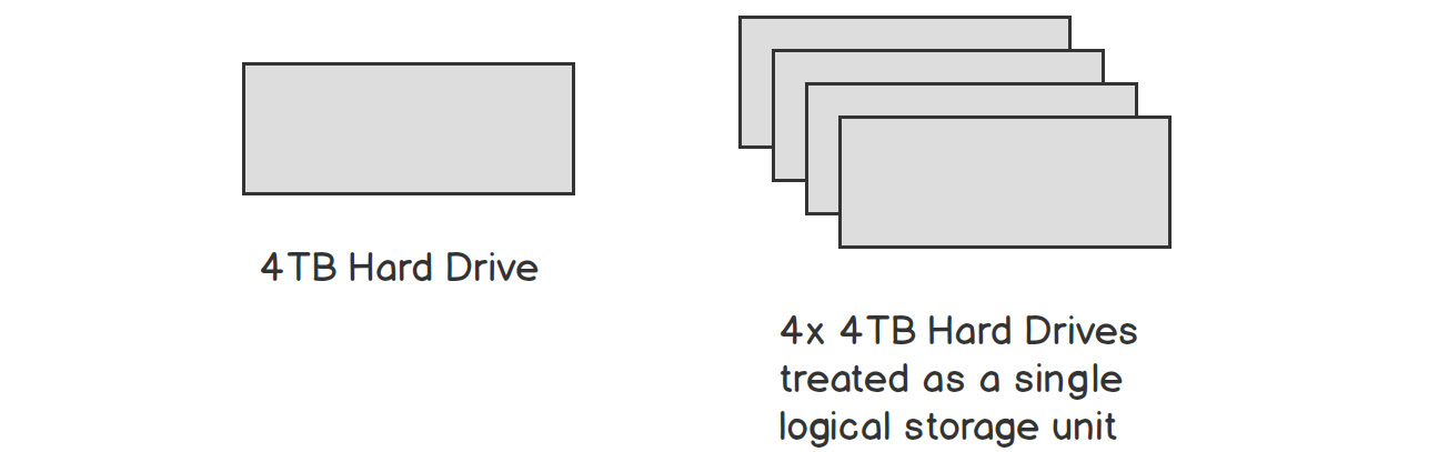
Figure 1.8: Linking units of hardware to simulate a larger storage capacity
As you work with larger and larger datasets, you will come across both horizontal and vertical scaling solutions, and it is important to understand when each is appropriate. Vertical scaling refers to adding more or better hardware to a single machine, and this is often the first way that scaling is attempted. If you find that you do not have enough RAM to run a particular algorithm on a particular dataset, it's often easy to try a machine that has more RAM. Similarly, for constraints in storage or processing capacity, it is often simple enough to add a bigger hard drive or a more powerful processor.
At some point, you will be using the most powerful hardware that money can buy, and it will be important to look at horizontal scaling. This refers to adding more machines of the same type and using them in conjunction with each other by working in parallel or sharing work and load in sophisticated ways.
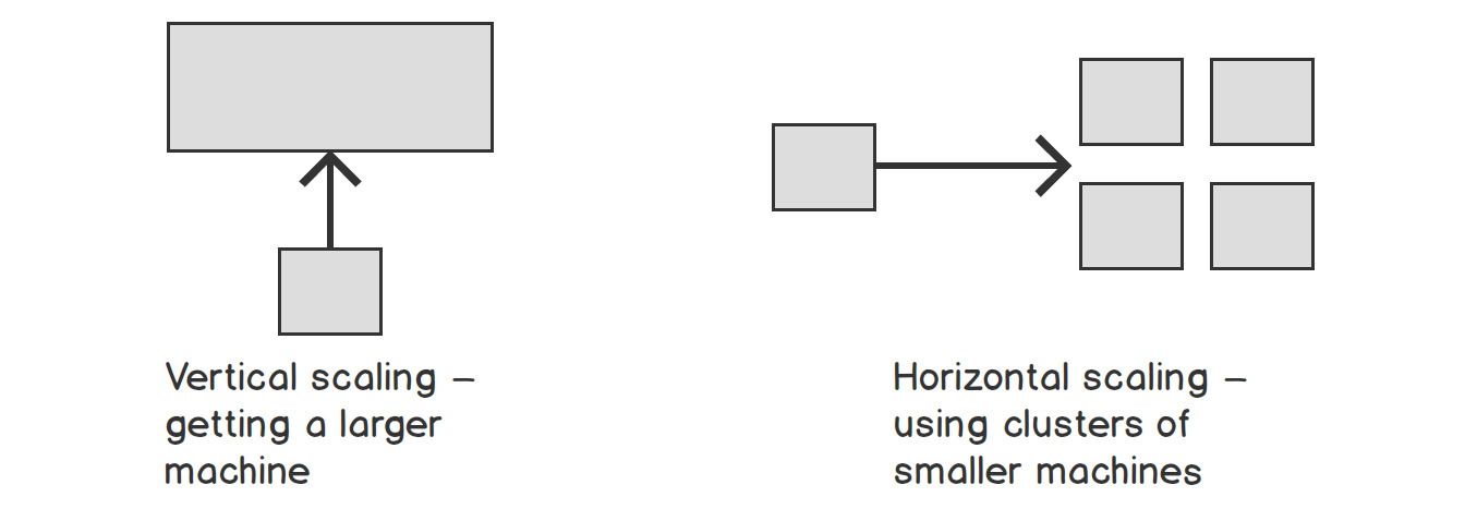
Figure 1.9: Vertical and horizontal scaling
Once again, cloud services can help us abstract away many of these problems, and most cloud services offer both virtual databases and so-called Binary Large Object (BLOB) storage. You will gain hands-on experience with both in later chapters of this book.
Optimizing hardware to be as powerful as possible is often important, but it also comes at a cost. Cost optimization is another important factor in optimizing systems.
Optimizing Cloud Costs – Spot Instances and Reserved Instances
Cloud services have made it much easier to rent specialized hardware for short periods, instead of spending large amounts of capital upfront during research and development phases. Companies such as Amazon (with AWS), Google (with GCP), and Microsoft (with Azure) allow you to rent virtual hardware and pay by the hour, so it is feasible to spin up a powerful machine and train your machine learning models in several hours, instead of waiting days or weeks for your laptop to crunch the numbers.
There are two important cost optimizations to be aware of when renting hardware from popular cloud providers: either by renting hardware for a very short time or by committing to rent it for a very long time. Specifically, because most cloud providers have some amount of unused hardware at any given moment, they usually auction it for short-term use.
For example, Amazon Web Services (AWS), the largest cloud provider currently, offers spot instances. If they have virtual machines attached to GPUs that no one has bought, you can take part in a live auction to use these machines temporarily at the fraction of the usual cost. This is often very useful for training machine learning models as the training can take place in a few hours or days, and it does not matter if there is a small delay in the beginning while you wait for an optimal price in the auction.
On the other side of the optimization scale, if you know that you are going to be using a specific kind of hardware for several years, you can usually optimize costs by making an upfront commitment about how long you will rent it. For AWS, these are termed reserved instances, and if you commit to renting a machine for 1, 2, or 3 years, you will pay less per hour than the standard hourly rate (though in most cases still more than the spot rate described previously).
In cases when you know you will run your system for many years, a reserved instance often makes sense. If you are training a model over a few hours or even days, spot instances can be very useful.
That's enough theory for now. Let's take a look at how we can practically use some of these optimizations. Because it is difficult to go out and buy expensive hardware just to learn about optimizations, we will focus on the optimizations offered by modern processors: vectorized operations.
Using Vectorized Operations to Analyze Data Fast
The core building blocks in all programmers' toolboxes are looping and conditionals – usually materialized as a for loop or an if statement respectively. Almost any programming problem in its most fundamental form can be broken down into a series of conditional operations (only do something if a specific condition is met) and a series of iterative operations (carry on doing the same thing until a condition is met).
In machine learning, vectors, matrices, and tensors become the basic building blocks, taking over from arrays and linked lists. When we are manipulating and analyzing matrices, we often want to apply a single operation or function to the entire matrix.
Programmers coming from a traditional computer science background will often use a for loop or a while loop to do this kind of analysis or manipulation, but they are inefficient.
Instead, it is important to become comfortable with vectorized operations. Nearly all modern processors support efficiently modifying matrices and vectors in parallel by executing the same operation to each element simultaneously.
Similarly, many software packages are optimized for exactly this use case: applying the same operator to many rows of a matrix.
But if you are used to writing for loops, it can be difficult to get out of the habit. So, we will compare the for loop with the vectorized operation to help you understand the reason to avoid using a for loop. In the next exercise, we'll use our headlines dataset again and do some basic analysis. We'll do each piece of analysis twice: first using a for loop, and then again using a vectorized operation. You'll see the speed differences even on this relatively small dataset, but these differences will be even more important on the larger datasets that we previously discussed.
While some languages have great support for vectorized operations out of the box, Python relies mainly on third-party libraries to take advantage of these. We'll be using pandas in the upcoming exercise.
Exercise 1.02: Applying Vectorized Operations to Entire Matrices
In this exercise, we'll use the pandas library to load the same clickbait dataset and we'll carry out some descriptive analysis. We'll do each piece of analysis twice to see the efficiency gains of using vectorized operations compared to for loops.
Perform the following steps to complete the exercise:
- Create a new directory, Exercise01.02, in the Chapter01 directory to store the files for this exercise.
- Open your Terminal (macOS or Linux) or Command Prompt (Windows), navigate to the Chapter01 directory, and type jupyter notebook.
- In the Jupyter notebook, click the Exercise01.02 directory and create a new notebook file with a Python3 kernel.
- Import the pandas library and use it to read the dataset file into a DataFrame, as shown in the following code:
import pandas as pd
df = pd.read_csv("../Datasets/clickbait-headlines.tsv",
sep=" ", names=["Headline", "Label"])
df
You should get the following output:
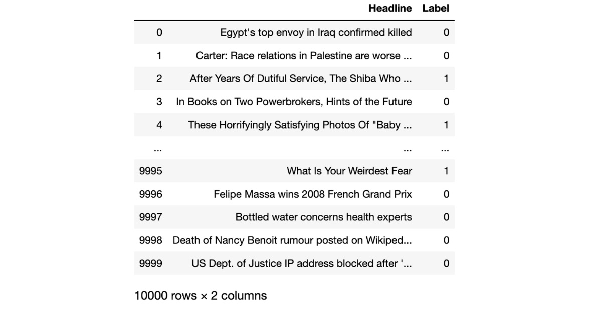
Figure 1.10: Sample of the dataset in a pandas DataFrame
We import the pandas library and then use the read_csv() function to read the file into a DataFrame called df. We pass the sep argument to indicate that the file uses tab ( ) characters as separators and then pass in the column names as the names argument. The output is summarized to show only the first few entries and the last few, followed by a description of how many rows and columns there are in the entire DataFrame.
- Calculate the length of each headline and print out the first 10 lengths using a for loop, along with the total performance timing, as shown in the following code:
%%time
lengths = []
for i, row in df.iterrows():
lengths.append(len(row[0]))
print(lengths[:10])
You should get the following output:
[42, 60, 72, 49, 66, 51, 51, 58, 57, 76]
CPU times: user 1.82 s, sys: 50.8 ms, total: 1.87 s
Wall time: 1.95 s
We declare an empty array to store the lengths, then loop through each row in our DataFrame using the iterrows() method. We append the length of the first item of each row (the headline) to our array, and finally, print out the first 10 results.
- Now re-calculate the length of each row, but this time using vectorized operations, as shown in the following code:
%%time
lengths = df['Headline'].apply(len)
print(lengths[:10])
You should get the following output:
0 42
1 60
2 72
3 49
4 66
5 51
6 51
7 58
8 57
9 76
Name: Headline, dtype: int64
CPU times: user 6.31 ms, sys: 1.7 ms, total: 8.01 ms
Wall time: 7.76 ms
We use the apply() function to apply len to every row in our DataFrame, without a for loop. Then we print the results to verify they are the same as when we used the for loop. From the output, we can see the results are the same, but this time it took only 16.3 milliseconds instead of over 1 second to carry out all of these calculations. Now, let's try a different calculation.
- This time, find the average length of all clickbait headlines and compare this average to the length of normal headlines, as shown in the following code:
%%time
from statistics import mean
normal_lengths = []
clickbait_lengths = []
for i, row in df.iterrows():
if row[1] == 1: # clickbait
clickbait_lengths.append(len(row[0]))
else:
normal_lengths.append(len(row[0]))
print("Mean normal length is {}"
.format(mean(normal_lengths)))
print("Mean clickbait length is {}"
.format(mean(clickbait_lengths)))
Note
The # symbol in the code snippet above denotes a code comment. Comments are added into code to help explain specific bits of logic.
You should get the following output:
Mean normal length is 52.0322
Mean clickbait length is 55.6876
CPU times: user 1.91 s, sys: 40.7 ms, total: 1.95 s
Wall time: 2.03 s
We import the mean function from the statistics library. This time, we set up two empty arrays, one for the lengths of normal headlines and one for the lengths of clickbait headlines. We use the iterrows() function again to check every row and calculate the length, but this time store the result in one of our two arrays, based on whether the headline is clickbait or not. We then take the average of each array and print it out.
- Now recalculate this output using vectorized operations, as shown in the following code:
%%time
print(df[df["Label"] == 0]['Headline'].apply(len).mean())
print(df[df["Label"] == 1]['Headline'].apply(len).mean())
You should get the following output:
52.0322
55.6876
CPU times: user 10.5 ms, sys: 3.14 ms, total: 13.7 ms
Wall time: 14 ms
In each line, we look at only a subset of the DataFrame: first when the label is 0, and second when it is 1. We again apply the len function to each row that matches the condition and then take the average of the entire result. We confirm that the output is the same as before, but the overall time is in milliseconds in this case.
- As a final test, calculate how often the word "you" appears in each kind of headline, as shown in the following code:
%%time
from statistics import mean
normal_yous = 0
clickbait_yous = 0
for i, row in df.iterrows():
num_yous = row[0].lower().count("you")
if row[1] == 1: # clickbait
clickbait_yous += num_yous
else:
normal_yous += num_yous
print("Total 'you's in normal headlines {}".format(normal_yous))
print("Total 'you's in clickbait headlines {}".format(clickbait_yous))
You should get the following output:
Total 'you's in normal headlines 43
Total 'you's in clickbait headlines 2527
CPU times: user 1.48 s, sys: 8.84 ms, total: 1.49 s
Wall time: 1.53 s
We define two variables, normal_yous and clickbait_yous, to count the total occurrences of the word you in each class of headline. We loop through the entire dataset again using a for loop and the iterrows() function. For each row, we use the count() function to count how often the word you appear and then add this total to the relevant total. Finally, we print out both results, seeing that you appear very often in clickbait headlines, but hardly in non-clickbait headlines.
- Rerun the same analysis without using a for loop and compare the time, as shown in the following code:
%%time
print(df[df["Label"] == 0]['Headline']
.apply(lambda x: x.lower().count("you")).sum())
print(df[df["Label"] == 1]['Headline']
.apply(lambda x: x.lower().count("you")).sum())
You should get the following output:
43
2527
CPU times: user 20.8 ms, sys: 1.32 ms, total: 22.1 ms
Wall time: 27.9 ms
We break the dataset into two subsets and apply the same operation to each. This time, our function is a bit more complicated than the len function we used before, so we define an anonymous function inline using lambda. We lowercase each headline and count how often "you" appears and then sum the results. We notice that the performance time, in this case, is again in milliseconds.
Note
To access the source code for this specific section, please refer to https://packt.live/2OmyEE2.
In this exercise, the main takeaway we can see is that vectorized operations can be many times faster than using for loops. We also learned some interesting things about clickbait characteristics though. For example, the word "you" appears very often in clickbait headlines (2,527 times), but hardly ever in normal headlines (43 times). Clickbait headlines are also, on average, slightly longer than non-clickbait headlines.
Let's implement the concepts learned so far in the next activity.
Activity 1.01: Creating a Text Classifier for Movie Reviews
In this activity, we will create another text classifier. Instead of training a machine learning model to discriminate between clickbait headlines and normal headlines, we will train a similar classifier to discriminate between positive and negative movie reviews.
The objectives of our activity are as follows:
- Vectorize the text of IMDb movie reviews and label these as positive or negative.
- Train an SVM classifier to predict whether a movie review is positive or negative.
- Check how accurate our classifier is on a held-out test set.
- Evaluate our classifier on out-of-context data.
Note
We will be using some randomizers in this activity. It is helpful to set the global random seeds to ensure that the results you see are the same as in the examples. Sklearn uses the NumPy random seed, and we will also use the shuffle function from the built-in random library. You can ensure you see the same results by adding the following code:
import random
import numpy as np
random.seed(1337)
np.random.seed(1337)
We'll use the aclImdb dataset of 100,000 movie reviews from Internet Movie Database (IMDb) – 50,000 each for training and testing. Each dataset has 25,000 positive reviews and 25,000 negative ones, so this is a larger dataset than our headlines one. The dataset can be found in our GitHub repository at the following location: https://packt.live/2C72sBN
You need to download the aclImdb folder from the GitHub repository.
Dataset Citation: Andrew L. Maas, Raymond E. Daly, Peter T. Pham, Dan Huang, Andrew Y. Ng, and Christopher Potts. (2011). Learning Word Vectors for Sentiment Analysis. The 49th Annual Meeting of the Association for Computational Linguistics (ACL 2011).
In Exercise 1.01, Training a Machine Learning Model to Identify Clickbait Headlines, we had one file, with each line representing a different data item. Now we have a file for each data item, so keep in mind that we'll need to restructure some of our training code accordingly.
Note
The code and the resulting output for this exercise have been loaded in a Jupyter notebook that can be found at https://packt.live/3iWYZGH.
Perform the following steps to complete the activity:
- Import the os library and the random library, and define where our training and test data is stored using four variables: one for training_positive, one for training_negative, one for test_positive, and one for test_negative, each pointing at the respective dataset subdirectory.
- Define a read_dataset function that takes a path to a dataset and a label (either pos or neg) that reads the contents of each file in the given directory and adds these contents into a data structure that is a list of tuples. Each tuple contains both the text of the file and the label, pos or neg. An example is shown as follows. The actual data should be read from disk instead of being defined in code:
contents_labels = [('this is the text from one of the files', 'pos'), ('this is another text', 'pos')]
- Use the read_dataset function to read each dataset into its variable. You should have four variables in total: train_pos, train_neg, test_pos, and test_neg, each one of which is a list of tuples, containing the relative text and labels.
- Combine the train_pos and train_neg datasets. Do the same for the test_pos and test_neg datasets.
- Use the random.shuffle function to shuffle the train and test datasets separately. This gives us datasets where the training data is mixed up, instead of feeding all the positive and then all the negative examples to the classifier in order.
- Split each of the train and test datasets back into data and labels respectively. You should have four variables again called train_data, y_train, test_data, and y_test where the y prefix indicates that the respective array contains labels.
- Import TfidfVectorizer from sklearn, initialize an instance of it, fit the vectorizer on the training data, and vectorize both the training and testing data into the X_train and X_test variables respectively. Time how long this takes and print out the shape of the training vectors at the end.
- Again, find the execution time, import LinearSVC from sklearn and initialize an instance of it. Fit the SVM on the training data and training labels, and then generate predictions on the test data (X_test).
- Import accuracy_score and classification_report from sklearn and calculate the results of your predictions. You should get the following output:

Figure 1.11: Results – accuracy and the full report
- See how your classifier performs on data on different topics. Create two restaurant reviews as follows:
good_review = "The restaurant was really great! "
"I ate wonderful food and had a very good time"
bad_review = "The restaurant was awful. "
"The staff were rude and "
"the food was horrible. "
"I hated it"
- Now vectorize each using the same vectorizer and generate predictions for whether each one is negative or positive. Did your classifier guess correctly?
Now that we've built two machine learning models and gained some hands-on experience with vectorized operations, it's time to recap.
Note
The solution to this activity can be found on page 580.
Summary
In this chapter, we gained a high-level overview of what machine learning can be used for, starting with image processing, text processing, audio processing, and time series analysis examples. This was followed by a deeper dive into text classification where we built a text classifier to identify clickbait headlines. We then looked at how to scale AI systems, looking at different kinds of hardware and cost-optimization techniques. By using vectorized operations, we were able to gain hands-on experience with optimization. Finally, we shored up our text-classification skills by building a second text classifier to differentiate between positive and negative movie reviews.
In the next chapter, we will explore ways to store large amounts of data for AI systems, looking specifically at data warehouses and data lakes.