In this chapter, we will focus on the data preparation that has to be done before an AI project can start with model training and evaluation. You will practice ETL (Extract, Transform, and Load) or ELT (Extract, Load, and Transform), data cleaning, and any other data prep work that is commonly required by data engineers. We will cover batch jobs, streaming data ingestion, and feature engineering. By the end of this chapter, you will have knowledge and some hands-on experience of data preparation techniques.
Introduction
In the previous chapter, we discussed the layers of a data-driven system and explained the important storage requirements for each layer. The storage containers in the data layers of AI solutions serve one main purpose: to build and train models that can run in a production environment. In this chapter, we will discuss how to transfer data between the layers in a pipeline so that the data is prepared to be used to train a model to create an actual forecast (called the execution or scoring of the model).
In an Artificial Intelligence (AI) system, data is continuously updated. Once data enters the system via an upload, application program interface (API), or data stream, it has to be stored securely and typically goes through a few ETL steps. In systems that handle streaming data, the incoming data has to be directed into a stable and usable data pipeline. Data transformations have to be managed, scheduled, and orchestrated. Further, the lineage of the data has to be stored to trace back the origins of a data point in a report or application. This chapter explains all data preparation (sometimes called pre-processing) mechanisms that ensure raw data can be used for machine learning by data scientists. This is important since raw data is hardly in a form that can be used by models. We will elaborate on the architecture and technology as explained by the layered model in Chapter 1, Data Storage Fundamentals. To start with, let's dive into the details of ETL.
ETL
ETL is the standard term that is used for Extracting, Transforming, and Loading data. In traditional data warehousing systems, the entire data pipeline consists of multiple ETL steps that follow after each other to bring the data from the source to the target (usually a report on a dashboard). Let's explore this in more detail:
E: Data is extracted from a source. This can be a file, a database, or a direct call to an API or web service. Once loaded with a query, the data is kept in memory, ready to be transformed. For example, a daily export file from a source system that produces client orders is read every day at 01:00.
T: The data that was captured in memory during the extraction phase (or in the loading phase with ELT) is transformed using calculations, aggregations, and/or filters into a target dataset. For example, the customer order data is cleaned, enriched, and narrowed down per region.
L: The data that was transformed is loaded (stored) into a data store.
This completes an ETL step. Similarly, in ELT, all the extracted data gets stored in the data store and then later transformed.
The following figure is an example of a full data pipeline, from a source system to a trained model:

Figure 3.1: An example of a typical ETL data pipeline
In modern systems such as data lakes, the ETL chain is often replaced by ELT. Rather than having, say, five ETL steps, where data is slowly refined and made ready for analysis, from a raw format to a queryable form, all the data is loaded into one large data store. Then, a series of transformations that are mostly virtual (not stored on disk) runs directly on top of the stored data to produce a similar outcome for analytics. In this way, a gain in storage space and performance can be achieved since modern (cloud-based) storage systems are capable of handling massive amounts of data. The data pipeline becomes somewhat simpler, although the various T(Transform) steps still have to be managed as separate software pieces:

Figure 3.2: An example of an ELT data pipeline
In the remainder of this chapter, we will look in detail at the ETL and ELT steps. Use the text and exercises to form a good understanding of the possibilities for preparing your data. Remember that there is no silver bullet; every use case will have specific needs when it comes to data processing and storage. There are many tools and techniques that can be used to get data from A to B; pick the ones that suit your company best, and whatever you pick, never forget the best practices of software development, such as version control, test-driven development, clean code, documentation, and common sense.
Data Processing Techniques
In Chapter 2, Artificial Intelligence Storage Requirements, we discussed the layers of a modern data lake and the requirements and possible data storage options for each layer. It became clear that data has to be sent to different data stores to maximize the abilities of AI: building a historical overview and a high-performing queryable source. This means that some work needs to be done with the data before it's suitable for a machine learning model. These data transfers usually happen as ETL steps in a data pipeline. We'll dive into the specifics and possibilities of batch processing in the following paragraphs.
In databases, a transaction is a fixed set of instructions that either fail or succeed. Transactions are very useful for data processing since they are reliable and produce no undesirable outcomes. Use them when certain steps are related, or have to be done in a certain order. If a transaction is composed of a hundred steps and the last one fails, all the previous steps are either not executed or rolled back. Transactions that guarantee this are called atomic and consistent. If two transactions are executed at the same time on the same database, for example, updating a large table, they should not influence each other; this property is called isolation. Transactions also should be durable: a completed transaction cannot be undone. If the transactions of a database are guaranteed to be atomic, consistent, isolated, and durable, the database is ACID-compliant. The opposite is a database that is BASE: Basically Available, Soft state, Eventually consistent.
In many cases, building a simple script or another piece of software is enough to get data from A to B. Each infrastructure, tool, and environment has its way of copying and filtering data. Some examples of simple data processing are:
- Bash or PowerShell scripts
- Python scripts
- SQL scripts
There are also ways of processing data that are discouraged, for various reasons. Building an Excel macro in Visual Basic (VB) is one of those methods. It might work, but it's difficult to test, distribute, and scale. Whenever you want to keep it simple, remember that all the follow-up actions should also be simple. In the following exercise, you'll build a simple data transformation step on CSV files with a Bash script.
Note
If you are facing challenges installing PySpark on your system, refer the following link: https://medium.com/tinghaochen/how-to-install-pyspark-locally-94501eefe421.
Exercise 3.01: Creating a Simple ETL Bash Script
Note
This exercise requires the BASH shell which is available on Linux and Unix-based systems (including MacOS). If you have Windows 10, you can install the shell through Windows Subsystem for Linux (WSL). To install WSL, you can follow the instructions detailed in the following article: https://docs.microsoft.com/en-us/windows/wsl/install-win10.
In this exercise, we're going to write a simple Bash script that reads data from a file (extract), does some data filtering (transform), and writes it to a new file (load). From the dataset, we're only interested in movies that are currently available in a certain country, we'll filter out the other records and remove a set of columns. This filter is the data transformation step. We'll use the standard CSV parsing library GNU awk (gawk) to process the file. After filtering, we'll simply write the result to a new file on disk.
We will be using a sample dataset of Netflix movies and TV series that was collected from Flixable, which is a third-party Netflix search engine. The dataset can be found in our GitHub repository at the following location: https://packt.live/2C72sBN.
You can download the netflix_titles_nov_2019.csv file from the GitHub repository.
Before proceeding to the exercise, we need to install the gawk utility in the local dev environment. Please follow the instructions in the Preface.
Perform the following steps to complete the exercise:
- Create a directory called Chapter03 for all the exercises in this chapter. In the Chapter03 directory, create the Exercise03.01 directory to store the files for this exercise.
- Move the netflix_titles_nov_2019.csv file to the Exercise03.01 directory.
- Open your Terminal (macOS or Linux) or Command Prompt (Windows), navigate to the Chapter03 directory, and type jupyter notebook.
- Select the Exercise03.01 directory, then click on New -> Python3 to create a new Python 3 notebook.
Note
If you have not installed gawk from the Preface, then you can type the installation commands in the first cell of the Jupyter Notebook. They are not included in the steps.
- Read the file using the Bash head command with an exclamation mark (!), as shown in the following code:
!head netflix_titles_nov_2019.csv
Note
The ! sign at the start of the preceding step notifies that we can run the BASH head command in Jupyter Notebook. To run the same command in the command line shell directly, exclude the ! sign.
You should get the following output:

Figure 3.3: Contents of the file with Netflix titles
Note
The output of the Jupyter Notebook is not visible in GitHub. Please download the Jupyter Notebook file locally and execute it.
You might notice that some fields are delimited by double quotes ("), and in those fields are commas as well. We should not treat those commas as field separators.
- Open a text editor and create a file called netflix.awk in the Exercise3.01 directory.
- Write the following code inside the netflix.awk file:
BEGIN {
FS=","
}
{
print "NF = " NF
for (i = 1; i <= NF; i++) {
printf("#%d = %s ", i, $i)
}
}
This file will be used to parse the CSV file. In the BEGIN statement, we have specified the parameters: for now, we just state that the separator is a comma (FS=","). In the remaining section, we have specified the output of the script. It now shows how many fields there are per line (NF) and then lists all the values in a print statement. The gawk utility can parse files or receive input from the prompt.
- Send the first 10 lines of a file as input to the gawk command using the pipe command (|), as shown in the following code:
!head netflix_titles_nov_2019.csv | gawk -f netflix.awk
Note
This is only a temporary step, and so the output is not in the notebook on GitHub since we will make modifications to the awk file.
You should get the following output:
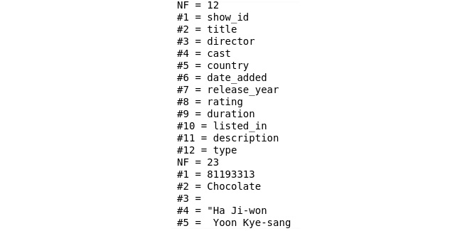
Figure 3.4: Output of the parsing of a comma-separated file with Netflix titles
As you can see, there is some comma-separation being done. We can see that there are 12 fields (NF=12) in the first line and the line contains the names of the fields as headers. However, the next line that is being parsed already contains 23 fields (NF=23). The reason is that the list of actors in the cast column contains commas as well. So, we can use the FPAT parameter instead of the FS parameter to gain more control over the separation of fields.
- Replace FS="," with FPAT = "([^,]+)|("[^"]+")" in the netflix.awk file, as shown in the following code:
BEGIN {
FPAT = "([^,]+)|("[^"]+")"
}
{
print "NF = " NF
for (i = 1; i <= NF; i++) {
printf("#%d = %s ", i, $i)
}
}
The FPAT parameter contains a regular expression that indicates what the contents of a field are. In our case, the fields are all text that is not a comma (indicated by ^,) or are delimited by double quotes (^"). For example, the string this is,"a test",and this,"also, right?" would split into the fields "this is", "a test", "and this", and "also, right?".
- Now check the output again by running the following command:
!head netflix_titles_nov_2019.csv | gawk -f netflix.awk
Note
This is only a temporary step and so the output is not in the notebook on GitHub since we will make modifications to the awk file.
You should get the following output:
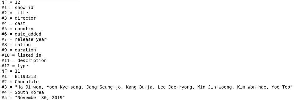
Figure 3.5: Output of the parsing of a comma-separated file with field delimiters
This output shows that the value in the cast column now is a comma-separated list of actors, just as expected. We also see double quotes in some values (for example, in the second line for the cast column), but we will leave them as-is for now.
There are two more things to fix. When looking at the data file and the output, you might notice that some lines contain less than 12 fields while there are 12 headers. The reason is that some fields in the source file are empty, resulting in commas next to each other (,,). This is something that we can easily change in our script by replacing all values of ,, with , , with a space in between the commas. Another peculiarity of the file is that quotes within quoted strings are represented with two double quotes (""). So, let's replace them with a single quote ('). There is a gsub() function within gawk that replaces all the instances of text with something else.
Note
The replacement will result in spaces for empty values; if at a later stage we decide on a different value to represent these null values, spaces can of course be changed to something else.
- Add gsub(",,", ", ,"), gsub(","""", ","'"), and gsub("""", "'") in the netflix.awk file, as shown in the following code:
BEGIN {
FPAT = "([^,]+)|("[^"]+")"
}
{
gsub(",,", ", ,")
gsub(","""", ","'")
gsub("""", "'")
print "NF = " NF
for (i = 1; i <= NF; i++) {
printf("#%d = %s ", i, $i)
}
}
- Now check the output again by running the following command:
!head netflix_titles_nov_2019.csv | gawk -f netflix.awk
Note
This is only a temporary step and so the output is not in the notebook on GitHub since we will make modifications to the awk file.
You should get the following output:

Figure 3.6: Output of the parsing of a comma-separated file with empty fields replaced and double quotes removed
You'll see that the output now has 12 columns for every line. With this step, we have completed our transformation step of ETL. This is great, but in the end, we don't want to get console output but rather filter the columns and write the output to a file. So, let's replace the print statement and the for loop in the script with the columns you want to have.
- To create a file with the show's title, year, rating, and type, add the following commands in the netflix.awk file:
BEGIN {
FPAT = "([^,]+)|("[^"]+")"
}
{
gsub(",,,,,", ", , , , ,")
gsub(",,,,", ", , , ,")
gsub(",,,", ", , ,")
gsub(",,", ", ,")
gsub(","""", ","'")
gsub("""", "'")
print $2","$7","$8","$12
}
Note
You can download the AWK file by visiting this link: https://packt.live/3ep6KBF.
The digits after the dollar signs refer to the indexes of the fields. In this example, we print the fields with numbers 2, 7, 8, and 12.
- Create a Bash script called parse.sh in the Exercise03.01 directory and add the following code:
head netflix_titles_nov_2019.csv | gawk -f netflix.awk
cat netflix_titles_nov_2019.csv| gawk -f netflix.awk >
netflix_filtered.csv
The Bash script sends its output to the disk. We have replaced the head (just the first 10 lines) of the file with the entire thing using the cat command. The pipe commands (|) send the input to the gawk command, and the > writes the output to a file.
- Open your Terminal (macOS or Linux) or Command Prompt window (Windows), navigate to the Chapter03/Exercise03.01 directory, and run the following command:
sh parse.sh
You should get the following output:
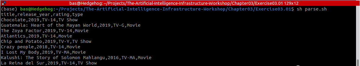
Figure 3.7: Output of the parse command that displays the top 10 Netflix titles and creates an output file
The data is stored in a CSV file named netflix_filtered.csv in the Exercise03.01 directory.
- Open the netflix_filtered.csv file in Jupyter Notebook using the following command:
!cat netflix_filtered.csv

Figure 3.8: Displaying the contents of the output file
Note
The output of the Jupyter Notebook is not visible in GitHub. Please download the Jupyter Notebook file locally and execute it.
We have successfully created a simple ETL Bash script.
Note
To access the source code for this specific section, please refer to https://packt.live/38TUKqA.
By completing this exercise, you processed a CSV file with some simple tools. We have shown that using a few standard Bash commands and an open CSV-parsing library is sometimes enough to process a file. At the same time, you have experienced that working with a simple CSV file is more complex than you would consider at first sight; trivial things such as empty values and quotes sometimes can be challenging. In the next paragraphs, we'll explore other methods of ETL that are suitable when simple scripting is not enough.
Traditional ETL with Dedicated Tooling
Many companies choose to acquire a software tool with the specific purpose of providing an ETL environment where batch jobs can be built, tested, and run in production. Examples of these tools include IBM DataStage, Informatica, Microsoft Azure Data Factory, and AWS Glue. Although these systems have their origin in the business intelligence and data warehousing domain, there is still a huge market for them. One of the benefits of these tools is that they provide a large collection of data transformations and connectors out of the box. After installation, the tools just work, and with a few configuration settings, developers can start creating ETL pipelines. They usually provide a rich graphical user interface with drag-n-drop functionality. There are also downsides to these tools. To truly understand them and work efficiently, engineers have to be trained and gain some experience with them. In the world of software engineering, this is often considered to be a too-specific career path. Rather than investing in skills for only one purpose (for example, ETL with a dedicated tool), many IT professionals consider it better to become senior in slightly more generic skills such as functional programming or database interfaces. Further, dedicated ETL tools such as DataStage and Informatica can become expensive since they are usually heavily licensed.
When choosing technology for data preparation and processing, it's worth a look inside your organization at existing ETL tools. Although it might feel more modern to write code in Python, Scala, or Go with a cool and hip framework, having a well-established team write an ETL job in a properly managed environment could be a more reasonable solution. Do bear in mind that these tools were often not created for scalability, portability, and performance in the big data and AI era.
As an alternative to traditional ETL with dedicated tooling, it's possible to write ETL in code. Many programming languages and frameworks are suited to this. In the next section, we'll focus on a modern big data engine that is popular for ETL: Apache Spark.
Distributed, Parallel Processing with Apache Spark
Over the past few years, data processing has become more and more important in enterprises as the size of data has grown tremendously. The term big data was coined around the year 2000 to indicate data where the volume, variety, or velocity was too large to handle with normal infrastructure and software. An important moment was the introduction and open-source publication of the Apache Hadoop framework, with which Yahoo! could store and process their massive amounts of data. Since then, the importance of big data and the amount of attention it attracts have grown tremendously. Companies such as Google, Facebook, and Alibaba continue to increase their data needs and have published papers and software about it. In the academic world, data analytics and machine learning have increased tremendously in popularity. We live in the big data era, which is impacting many organizations. For our evaluation of data processing methods, we can now consider a large set of tools and methods that help to make ETL processes possible even when dealing with big datasets.
Currently, Apache Spark is one of the leading big data frameworks, designed to allow massive data processing. It works by parallelizing data across the nodes of a cluster and executing tasks on the distributed data in memory. Spark quickly became one of the most popular data tools after Hadoop MapReduce, which is a slower and more low-level programming framework.
The main concept of Spark is the resilient distributed dataset (RDD). Since Spark 1.3, RDDs have evolved into DataFrames, and Spark 1.6 introduced the concept of Datasets. These are data structures that represent an RDD in a table-like format with rows and columns, making it even easier to work with big data.
The beauty of Spark is that it has an API that abstracts away the complexity of distributing data and bringing it back together again. Programming in Spark feels like ordinary (functional) programming, where functions such as map and filter can be applied to data collections. Only, with Spark, it doesn't matter if that data collection is 10 MB or 10 TB in size. You'll learn more about the concepts and workings of Spark in Chapter 7, Introduction to Analytics Engine (Spark) for Big Data. For now, we'll go through a simple exercise to get familiar with Spark for ETL.
Exercise 3.02: Building an ETL Job Using Spark
In this exercise, we'll use Spark to process the same dataset as used in Exercise 3.01, Creating a Simple ETL Bash Script. We'll download the data, apply a filter, transform a column into a machine-readable format, and store the resulting dataset on disk. This illustrates the process of writing ETL code in Spark. Since most of our examples in this book are programmed in Python, we will use the pyspark library, which uses Python to connect to Spark.
Note
In many cases, using Python might not be obvious since Spark is built in Scala. However, once you have learned the basics of Spark with PySpark, it's easy to switch to another programming language, such as Java or Scala.
Before proceeding to the exercise, we need to set up Java and PySpark in the local environment. Please follow the instructions in the Preface to install them.
Java is needed to run Spark since the Spark framework makes use of some standard Java libraries. It expects the java command to be available on your system, and the JAVA_HOME environment variable to be set. So, make sure that Oracle Java 8, 9, or 10 is installed on your system. Java 11 is not supported by Spark yet. Also, make sure that your JAVA_HOME environment variable is set; if not, do so by pointing it to your local Java folder, for example, export JAVA_HOME=/usr/lib/jvm/java-8-oracle.
Perform the following steps to complete the exercise:
- Create a directory called Exercise03.02 in the Chapter03 directory to store the files for this exercise.
- Open your Terminal (macOS or Linux) or Command Prompt (Windows), navigate to the Chapter03 directory, and type jupyter notebook.
- Select the Exercise03.02 directory, then click on New -> Python3 to create a new Python 3 notebook.
- First, you need to have Spark installed (link is provided in the Preface). You can then install PySpark by referring the Preface, or by running the following commands in a Jupyter Notebook cell.
import sys
!conda install --yes --prefix {sys.prefix}
-c conda-forge pyspark
You should get the following output:

Figure 3.9: Installing PySpark with Anaconda
Note
Alternatively, you can also install PySpark using the following command in Terminal (macOS or Linux) or Command Prompt (Windows):
pip install pyspark
- Connect to a Spark cluster or a local instance using the following code:
from pyspark.sql import SparkSession
from pyspark.sql.functions import col, split, size
spark = SparkSession.builder.appName("Packt").getOrCreate()
These commands produce no output if they are successful; you'll only see that the cell in the Jupyter Notebook has completed running.
The getOrCreate command of the SparkSession.builder object creates a new Spark session, which is the main context of a Spark job. When this code is run in a production environment, it might contain hundreds of servers. For now, it's just your laptop.
- Load and show the contents of the dataset in a Spark DataFrame using the following code:
data = spark.read.csv(
'../../Datasets/netflix_titles_nov_2019.csv',
header='true')
data.show()
Note
The CSV file used in the preceding step can be downloaded from https://packt.live/2C72sBN. Make sure you change the path (highlighted) based on where you have saved the file locally.
You should get the following output:

Figure 3.10: Reading data from a CSV file into a Spark DataFrame
The spark.read.csv command reads the contents of a CSV file into memory. The resulting object (data in our case) is a DataFrame, which is a distributed dataset that is available for querying and other analysis. Since we specified header='true' in the read.csv command, PySpark interprets the first line as the header of the dataset. Notice that the difficulties we had in Exercise 3.01, Creating a Simple ETL Bash Script, with separating the commas and quotes are handled by PySpark for us automatically. There are 12 columns as expected, and empty strings are denoted as null.
The data object now contains an in-memory representation of the dataset in a Spark DataFrame object (made visible in the data.show() statement). If you run this on a Spark cluster, the DataFrame will be distributed across the nodes
- Apply the data.filter() function to filter the movies of 2019, as shown in the following code:
movies = data.filter((col('type') == 'Movie')
& (col('release_year') == 2019))
movies.show()
You should get the following output:

Figure 3.11: Filtering a Spark DataFrame
- Transform the list of actors into a number to show how many main actors were listed in the dataset using the following code:
transformed = movies.withColumn(
'count_cast', size(split
(movies['cast'], ',')))
We have created a new column, 'count_cast'. To calculate it, we first split the string in the 'cast' column and then take the size of the resulting array; this counts the number of actors and saves it in the transformed variable. As the dataset contains a lot of columns, we will only select a few columns.
- Select a subset of columns for the 2019 movies using the following code:
selected = transformed.select('title', 'director',
'count_cast', 'cast', 'rating',
'release_year', 'type')
- Read the filtered data using the following code:
selected.show()
You should get the following output:

Figure 3.12: Transforming a Spark DataFrame
- Write the contents of our still in-memory DataFrame to a comma-separated file using the following code:
selected.write.csv('transformed' , header='true')
This produces a directory called transformed that contains some metadata and the actual output in CSV format. The output file has a name like part-00000-...csv. The first line of the output file contains the header since we specified header='true' in a similar way as when loading the source file.
Note
Alternatively, we can add the complete code of the ETL process so far in a Python script and run it through the Terminal (macOS or Linux) or Command Prompt (Windows). We have created the same spark_etl.py Python script at the following location: https://packt.live/2ATRPSt. Run this by opening a Terminal (macOS or Linux) or Command Prompt (Windows)or Anaconda Prompt in the same folder as the script and executing the following command: python spark_etl.py
- Open the comma-separated file in the transformed directory in Jupyter Notebook using the following command:
# note: the actual name of the csv file
#('part-....') differs on each run
!head transformed/part-00000-
96ee95ae-9a80-4e88-b876-7f73893c2f21-c000.csv
Note
The aforementioned command will only work on Linux and UNIX-based systems. On Windows, you can browse the same file via Windows Explorer.
You should get the following output:

Figure 3.13: CSV file in the transformed directory
Note
To access the source code for this specific section, please refer to https://packt.live/308Xahr.
You have now completed a simple exercise that demonstrates the power of Spark when it comes to working with data. If you choose to write your ETL as source code, Spark can be considered a good option for large datasets. When working with a Spark DataFrame (or DataSet) object, many more transformations are possible: grouping data, aggregation, and so on. It's even possible to write SQL queries on the data. We will learn about these in more detail in Chapter 7, Introduction to Analytics Engine (Spark) for Big Data. In the next activity, you'll write an ETL job with Spark in a business-like scenario.
Activity 3.01: Using PySpark for a Simple ETL Job to Find Netflix Shows for All Ages
You work for a kids' TV channel and plan to launch a new show. You want a list of Netflix shows for 2019 that are for all ages, along with their ratings and other details. Based on the details, you will work on your new show.
In this activity, you'll load the Netflix dataset, filter the shows based on parental guidelines, and store the result in a CSV file.
Note
The code and the resulting output for this activity have been loaded in a Jupyter Notebook that can be found here: https://packt.live/3iXSinP.
Perform the following steps to complete the activity:
- Create a Python file or Jupyter Notebook.
- Connect to a local Spark cluster by importing the PySpark libraries and building a SparkSession object.
- Read the CSV file, netflix_titles_nov_2019.csv, from disk, and load it into a Spark DataFrame.
- Filter the data: select only the TV shows where the rating is either TV-G (for all ages) or TV-Y (for children). You should get the following output:

Figure 3.14: The contents of the file with TV shows filtered by rating
- Add a new column called count_lists, which contains the number of lists that are in the listed_in column.
- Select the title, count_directors, director, cast, rating, release_year, duration, listed_in, and description columns.
- Write the output of the filtered data to a comma-separated file ('transformed2.csv').
- View the CSV file to get the following output:
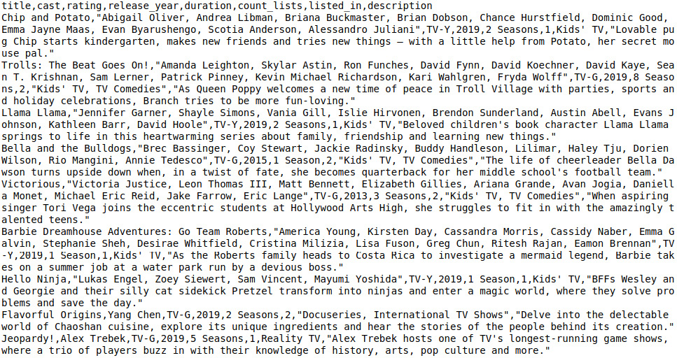
Figure 3.15: CSV file in the transformed2 directory
You now have a general understanding of data processing techniques that can be used for any ETL step. You have learned about simple scripts, ETL tools, and Spark. In the remainder of this chapter, we will do a deep dive into each ETL step. Each section refers to one of the steps in the pipeline shown in Figure 3.1. We'll start with the first step: importing raw data from a source system.
Note
The solution to this activity can be found on page 587.
Source to Raw: Importing Data from Source Systems
Typically, data comes to an AI system in the form of files. This may sound old-fashioned, but the truth is that this kind of data transfer is still very effective and universal. Almost all core systems of an organization can export their data in some form, whether CSV, Excel, XML, JSON, or something else. More modern ways to produce batch data are via on-demand APIs that query a system with parameters. However, this way of interfacing is sometimes not the highest priority for software builders.
They understand that systems have to interact and thus provide some form of interface, but it's not in their interests to make it very easy to get data from the system. Moreover, it's expensive to document and maintain an API once it's developed; once consumers rely on the connection, any change has to be managed carefully. Since many core systems are built on standard technology such as a relational database (Oracle, SQL Server, PostgreSQL, MySQL, and so on) and these databases have built-in features to export data already, it's tempting to simply utilize these features rather than to build custom APIs that require software engineering, testing, and management. So, although APIs provide a more stable and robust way of getting data, file transfers are a major way of interacting with source systems and it's not likely that a quick shift will happen in the near future. We often deal with legacy systems or vendor products and cannot influence the way that this software works.
After importing the raw data from a source file, the next step in an ETL pipeline is to clean it. Let's explore that topic in the next section.
Raw to Historical: Cleaning Data
One of the most important tasks for a data engineer who works on AI solutions is cleaning the data. Raw data is notoriously dirty, by which we mean that it's not suitable for use in a model or any other form of consumption, such as displaying on a website. Dirty data can have many forms:
- Missing values, such as null values or empty strings
- Inconsistent values, such as the string "007" where integers are expected
- Inaccurate values, such as a date with a value of 31 February 2018
- Incomplete values, such as the string "Customer 9182 has arri"; this can be due to limited field lengths
- Unreadable values, such as "K/dsk2#ksd%9Zs|aw23k4lj0@#$" where a name is expected; this can be due to encryption where it's not expected or wrong data formats (Unicode, UTF-8, and so on)
The ideal point to clean data is when data is processed from the raw data layer into the historical data layer. After all, the historical archive functions as the one version of the truth and should contain ready-to-use records. But we have seen many times that data needs a bit more cleaning, even after querying it from the historical layer or the analytics layer. This can be due to sloppy ETL developers or other reasons. It might also be on purpose; a conscious decision might have been made by management as part of a trade-off discussion to keep the data in a somewhat raw/dirty format since cleaning it simply takes a lot of time and effort.
The way to clean data is to write code that transforms the dirty data into the proper format and values. There is no one good data format or data model; it depends on the organization and use case. Some people might prefer a date-time format of YYYY-MM-DD, while others prefer MM-DD-YYYY. Some might allow storing null values, while others require a value, for example, an empty string or default integer. What's important is to make choices, to document them, to communicate them clearly, and to check them. Code that cleans data can be shared and reused among developers to make the work easier and to standardize the outcomes.
The next step in an ETL pipeline is modeling the data. We'll cover that in the next section.
Raw to Historical: Modeling Data
To transform raw data into a form that can be stored in a historical archive, some steps need to be taken depending on the shape of the raw data and the chosen target model. Raw data should be modeled into a shape so that is can be stored for historical analysis. The raw data usually resides in files and has to be mapped to relational database tables. A typical process is to read a CSV file, transform the data in memory, and write the transformed data to a database where the tables are created in the fashion of a data vault. A data vault is a relational model intended for data warehousing, developed by Dan Linstedt. Other popular target models that offer normalized data models are the Dimensional Data Mart (DDM) approach by Ralph Kimball and the Corporate Information Factory (CIF) by Bill Inmon.
After modeling the data and creating a historical archive, it's time to start preparing the data for analysis by building up the analytics layer with ETL jobs. The following paragraphs contain two important steps in that phase: filtering and aggregation, and flattening the data.
Historical to Analytics: Filtering and Aggregating Data
Not all the data in a historical archive will be needed in the analytics layer. Therefore, a filter has to be applied, for example, to only take the data of the past year. This is needed to further reduce the amount of data that is stored in the analytics layer and improve query performance. Some fields can be aggregated (for example, sums, summaries, and averages).
Historical to Analytics: Flattening Data
A technique to make data available for efficient querying in the analytics layer of a data-driven solution is to flatten it. Flattening data means to let go of the normalized form of the Linstedt/Kimball/Inmon tables and create one big table with many columns, where some data is repeated instead of being stored in foreign keys.
When an analytics layer is created, the data is prepared for consumption by a machine learning model. The following section explores an important step that is still considered to be part of the ETL pipeline: feature engineering.
Analytics to Model: Feature Engineering
The final step in preparing the data for machine learning model development and training is to transform the data records so that the models can consume them. This transformation into model-readable data is called feature engineering. Features are the characteristics of a dataset by which a predictive model can be evaluated. A good feature has a lot of predictive power; knowing the value of such a feature gives us immediate results in terms of the predictability of the outcome of a model. For example, if we have a dataset with 100,000 people and have to predict which language each person speaks, a very indicative feature will be the country of residence. In the same dataset, the height or age of the person will be weak features for the language detection algorithm.
Features can be stored in a dedicated feature store, which is part of the analytics layer in a modern data lake. The feature store is just a database that is easy to query when working with machine learning models. It can be considered the final data store in an ETL or ELT pipeline, where the final T step is feature engineering. Features can also be exported to disk as part of the model's code.
Features play an important role in two stages of a machine learning project:
- While developing and training the model, all training data has to be transformed into a feature set. This is called feature engineering.
- While running in production and executing/scoring the model, new data that comes in and has to be analyzed by the model has to go through the same feature transformation steps.
The code that transforms the source data into features, therefore, has to be deployed to two locations: the machine learning environment and the production environment. The source code in these two places has to be the same, otherwise, the trained models will produce different results than the models in production. Therefore, it's important to carefully maintain and manage this code. Version control, continuous delivery, documentation, and monitoring are all best practices that ensure that no mistakes are made. A good way to ensure consistency is to store the models together with the feature engineering code; they belong together and thus should have the same version, release plan, and documentation.
Features can be derived in four ways. A column with features in a dataset for model training can have one of the following origins:
- Data column: Data that feeds a model may already be in the right shape.
- The translation of one source column, for example, the usage of the number in the age column in a dataset of people.
- The combination of other columns, for example, the sum of all values in three source columns with product prices.
- From an external source: Sometimes, the data in a source column only contains a reference or pointer to an external data source. In those cases, a query has to be made to an external system, for example, a cache database with customer records or an API call to a core system. This will introduce a dependency on an external resource, which has to be managed and monitored. Since this step is resource-intensive, especially for large datasets, it's also crucial to carefully test the performance.
In many cases, depending on the choice of the machine learning algorithm, features have to be normalized. This is the process of getting numerical features in the same order of magnitude to be able to optimize the algorithm. The usual practice is to bring all numbers into the range 0 to 1 by looking at the minimum and maximum values that are in a dataset. For example, the values in the height column of a dataset of people might initially range from 45 to 203 centimeters. By executing the function h → (h - 45) / 158 on each value h, all values will range from 0 (the initial 45 cm) to 1 (the initial 203 cm).
Alongside feature engineering, it's important to split a dataset for training and testing models. We'll explore that topic in the next section.
Analytics to Model: Splitting Data
The final data preparation step in a data pipeline is to split the data in a train and test dataset. If you have a big dataset, a model needs to be trained on only a part of it (for example, 70%). The remainder of the same dataset (30%) is kept aside for validating or testing the model. Common ratios are in the range of 80-20 to 70-30. It's essential that the datasets for training and testing are both from the same original dataset, and that the division is done randomly. Otherwise, it's possible that the model will be overfitted to the training dataset and the results on the test dataset (and all other forthcoming predictions) will not be accurate or precise.
The work of splitting the original dataset is usually done by a data scientist. All modern data frameworks and tools contain methods to do this. For example, the following code is for splitting a dataset in the popular Python framework scikit-learn:
from sklearn.model_selection import train_test_split
X_train, X_test,
Y_train, Y_test = train_test_split(X, y,
test_size=0.25, random_state=42)
In the preceding statement, the train_test_split function is called. This function is a standard method in the Python scikit-learn (sklearn) library to split a dataset (X) with output variables (y) into a random training part and a random testing part. The training set is called X_train, and the output variables are in Y_train, and they contain 100% – 25% = 75% of the data.
Streaming Data
This chapter so far has explored data preparation methods for batch-driven ETL. You have learned the steps and techniques to get raw data from a source system, transform it into a historical archive, create an analytics layer, and finally do feature engineering and data splitting. We'll now make a switch to streaming data. Many of the concepts you have learned for batch processing are also relevant for stream processing; however, things (data) move a bit more quickly and timing becomes important.
When preparing streaming event data for analytics, for example, to be used in a model, some specific mechanisms come into play. Essentially, a data stream goes through the same steps as raw batch data: it has to be loaded, modeled, cleaned, and filtered. However, a data stream has no beginning and ending, and time is always important; therefore, the following patterns and practices need to be applied:
- Windows
- Event time
- Watermarks
We'll explain these topics in the next sections.
Windows
In many use cases, it's not possible to process all the data of a never-ending stream. In those cases, it is required to split up the data stream into chunks of time. We call these chunks windows of time. To window a data stream means to split it up into manageable pieces, for example, one chunk per hour.
There are several types of windows:
- A tumbling window has a fixed length and does not overlap with other windows. Events (the individual records) in a stream with tumbling windows only belong to one window.
- A sliding window has a fixed length but overlaps other sliding windows for a certain duration. Events in a stream with sliding windows belong to multiple windows since one window will not be completed yet when other windows begin. The window size is the length of the window; the window slide determines the frequency of windows.
- A session window is a window that is defined by the events themselves. The start and end of a session window are determined by data fields, for example, the login and log out actions of a website. It's also possible to define session windows by a series of following events with a gap in between. Session windows can overlap, but events in a stream with session windows can only belong to one session.
The following figure displays these kinds of windows in an overview. Each rectangle depicts a window that is evaluated in the progression of time. Each circle represents an event that occurred at a certain moment in time. For example, the first tumbling window contains two events, labeled 1 and 2. It's clear to see that sliding windows and session windows are more complex to manage than tumbling windows: events can belong to multiple windows and it's not always clear to which window an event belongs.

Figure 3.16: Different types of time windows for streaming data
Modern stream processing frameworks such as Apache Spark Structured Streaming and Apache Flink provide built-in mechanisms for windowing, and customizable code to allow you to define your time windows.
While windowing the data in your stream is not necessary, it provides a great way to work with streaming data.
Event Time
It's important to realize that events contain multiple timestamps. We can identify three important ones:
- The event time: The timestamp that the event occurs. For example, the moment a person clicks on a button on a web page (say, at 291 milliseconds after 16:45).
- The ingestion time: The timestamp at which the event enters the stream processing software engine. This is slightly later than the event time since the event has to travel across the network and perhaps a few data stores (for example, a message bus such as Kafka). An example of the ingestion time is the moment that the mouse-click of the customer enters the stream processing engine (say, at 302 milliseconds after 16:45).
- The processing time: The timestamp at which the event is evaluated by the software that runs as a job within the stream processing engine. For example, the moment that the mouse-click is compared to the previous mouse-click in a window, to determine whether a customer is moving to another section of a website (say, at 312 milliseconds after 16:45).
In most event data, the event time is included as a data field. For example, money transactions contain the actual date and time when the transfer was made. This should be fairly accurate and precise, for example, in the order of milliseconds. The processing time is also available in the data stream processor; it's just the server time, defined by the clock of the infrastructure where the software runs. The ingestion time is somewhat rare and hardly used; it might be included as an extra field in events if you know that the processing of events takes a long time and you want to perform performance tests.
When analyzing events, the event time is the most useful timestamp to work with. It's the most accurate indication of the event. When the order of events is important, the event time is the only timestamp that guarantees the right order, since latency can cause out-of-order effects, as shown in the following figure:

Figure 3.17: The timestamps and out-of-order effects in a data stream
In Figure 3.17 the dark blue circles represent timestamps. The blue arrows indicate the differences in time between the timestamps. For each event, event time always occurs first, followed by the ingestion time, and finally the processing time. Since these latencies can differ per event, as indicated by the highlighted circles, the out-of-order effect can occur.
Late Events and Watermarks
At the end of each window, the events in that window are evaluated. They can be processed as a batch in a similar way as normal ETL processes: filtering, enriching, modeling, aggregating, and so on. But the end of a window is an arbitrary thing. There should be a timed trigger that tells the data stream processor to start evaluating the window. For that trigger, the software could look at the processing time (its server clock). Or, it could look at the event data that comes in and trigger the window evaluation once an event comes in with a timestamp that belongs to the next window. All these methods are slightly flawed; after all, we want to look at the event time, which might be very different from the processing time due to network latency. So, we can never be sure that a trigger is timed well; there might always be events arriving in the data stream that belong to the previous window. They just happened to arrive a bit later. To cater to this, the concept of watermarking was introduced.
A watermark is an event that triggers the calculation of a window. It sets the evaluation time for the window a bit later than the actual end-time of the window, to allow late events to arrive. This bit of slack is all that is needed to make sure that most of the events are evaluated in the right window where they belong, and not in the next window or even ignored (see Figure 3.18).

Figure 3.18: Late events that are still evaluated in the correct window based on their event time
In the next exercise, you'll build a stream processing job with Spark where the concepts of windows, event time, and watermarks are used.
Exercise 3.03: Streaming Data Processing with Spark
In this exercise, we are going to connect to a data stream and process the events. You'll connect to a real Twitter feed and aggregate the incoming data by specifying a window and counting the number of tweets. We'll use the Spark Structured Streaming library, which is rich in functionality and easy to use.
Since we are going to connect to Twitter, you'll need a Twitter developer account:
- Go to https://developer.twitter.com/ and create an account (or log in with your regular Twitter account if you already have one).
- Apply for an API by clicking Apply and selecting the purpose of Exploring the API.
- Fill in the form where you have to state the usage of Twitter data.
- After approval, you'll see an app in the Apps menu. Select the new app and navigate to the Keys and tokens tab. Click Generate to generate your access token and secret. Copy these and store them in a safe location, for example, a local file.
- Click Close and also copy the API key and API secret key in the local file. Never store these on the internet or in source code.
- Make sure that Oracle Java 8, 9, or 10 is installed on your system. Java 11 is not supported by Spark yet. Also, make sure that your JAVA_HOME environment variable is set; if not, do so by pointing it to your local Java folder, for example, export JAVA_HOME=/usr/lib/jvm/java-8-oracle.
- We'll use the tweepy library to connect to Twitter. Get it by following the installation instructions in the Preface.
There are two parts to this exercise. First, we will connect to Twitter and get a stream of tweets. We'll write them to a local socket. This is not supported for production, but it will do fine in a local development scenario. In production, it's common to write the raw event data to a message bus such as Kafka.
Perform the following steps to complete the exercise:
- Create a new Python file in your favorite editor (for example, PyCharm or VS Code) or a Jupyter Notebook and name it get_tweets.py or get_tweets.ipynb.
- If you're using Jupyter Notebook, install the tweepy library by entering the following lines in a cell and running it:
import sys
!conda install --yes --
prefix {sys.prefix} -c conda-forge tweepy
- If you're using an IDE, make sure that tweepy is installed by typing the following command in your Anaconda console or shell:
pip install tweepy
- Connect to the Twitter API by entering the following code:
import socket
import tweepy
from tweepy import OAuthHandler
# TODO: replace the tokens and secrets with your own Twitter API values
ACCESS_TOKEN = ''
ACCESS_SECRET = ''
CONSUMER_KEY = ''
CONSUMER_SECRET = ''
Replace the values in the strings with the keys and secrets that you wrote down in the preparation part of this exercise.
- To connect to Twitter, the tweepy library first requires us to log in with the Oauth credentials that are in the keys and secrets. Let's create a dedicated method for this:
def connect_to_twitter():
auth = OAuthHandler(CONSUMER_KEY, CONSUMER_SECRET)
auth.set_access_token(ACCESS_TOKEN, ACCESS_SECRET)
api = tweepy.API(auth)
- Now let's handle the events by adding some lines to the connect_to_twitter function. Put the following lines in the cell with the connect_to_twitter function:
my_stream_listener = MyStreamListener()
my_stream = tweepy.Stream(auth=api.auth, listener=my_stream_listener)
# select a (limited) tweet stream
my_stream.filter(track=['#AI'])
The connect_to_twitter function now authenticates us at the Twitter API, hooks up the MyStreamListener event handler, which sends data to the socket and starts receiving data from Twitter in a stream with the #AI search keyword. This will produce a limited stream of events since the Twitter API will only pass through a small subset of the actual tweets.
- Next, the tweepy library needs us to inherit the StreamListener class. We have to specify what to do when a tweet comes in an override of the on_data() function. In our case, we send all data (the entire tweet in JSON format) to the local socket:
class MyStreamListener(tweepy.StreamListener):
def on_error(self, status_code):
if status_code == 420:
return False
def on_data(self, data):
print(data)
# send the entire tweet to the socket on localhost where pySpark is listening
client_socket.sendall(bytes(data, encoding='utf-8'))
return True
We will now set up a local socket that has to be connected to Twitter. Python has a library called socket for this, which we imported already at the top of our file.
- Write the following lines to set up a socket at port 1234:
s = socket.socket()
s.bind(("localhost", 1234))
print("Waiting for connection...")
s.listen(1)
client_socket, address = s.accept()
print("Received request from: " + str(address))
- The final step is to call the connect_to_twitter method at the end of the file. We are still editing the same file in the IDE; add the following lines at the end:
# now that we have a connection to pySpark, connect to Twitter
connect_to_twitter()
- Run the get_tweets.py file from a Terminal (macOS or Linux) or Command Prompt (Windows)or Anaconda Prompt using the following command:
python get_tweets.py
You should get the following output:
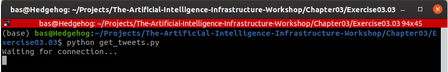
Figure 3.19: Setting up a connection to the Twitter API from a terminal
The first part is now done. Run this file to set up the socket and the connection to Twitter. If all is well, there will be a Python job running with no output but Waiting for connection…. Since the socket has to respond to a caller, we have to create a socket client that listens to the same port.
The next part is to connect a Spark job to the socket on localhost (or a Kafka topic in production), get the tweets as a data stream, and perform a window operation on them.
- Create a new Python file or Jupyter Notebook and name it spark_twitter.py or spark_twitter.ipynb.
Note
The spark_twitter Jupyter Notebook can be found here:
- If you have done Exercise 3.02, Building an ETL Job Using Spark, PySpark is already installed on your local machine. If not, install PySpark with the following lines:
import sys
!conda install --yes --prefix {sys.prefix}
-c conda-forge pyspark
- We first have to connect to a Spark cluster or a local instance. Enter the following lines in the file, notebook, or Python shell:
from pyspark.sql import SparkSession
from pyspark.sql.functions import from_json,
window, to_timestamp
from pyspark.sql.types import StructType,
StructField, StringType
- Enter the following line to create a Spark session:
spark = SparkSession.builder.appName('Packt').getOrCreate()
- To connect to the socket on localhost, enter the following line:
raw_stream = spark.readStream.format('socket')
.option('host', 'localhost')
.option('port', 1234).load()
Now, we have a stream of raw strings. These should be converted from JSON to a useful format, namely, a text field with the tweet text and a timestamp field that contains the event time. Let's do that in the next step.
- We'll define the JSON schema and add the string format that Twitter uses for its timestamps:
tweet_datetime_format = 'EEE MMM dd HH:mm:ss ZZZZ yyyy'
schema = StructType([StructField('created_at',
StringType(), True),
StructField('text', StringType(), True)])
- We can now convert the JSON strings with the from_json PySpark function:
tweet_stream = raw_stream.select(from_json('value', schema).alias('tweet'))
- The created_at field is still a string, so we have to convert it to a timestamp with the to_timestamp function:
timed_stream = tweet_stream
.select(to_timestamp('tweet.created_at',
tweet_datetime_format)
.alias('timestamp'),
'tweet.text')
- At this moment, you might want to check whether you're receiving the tweets and doing the parsing right. Add the following code:
query = timed_stream.writeStream.outputMode('append')
.format('console').start()
query.awaitTermination()
Note
This function is not complete yet. We'll add some code to it in the next step.
- Run the file on a Terminal (macOS or Linux) or Command Prompt (Windows) or Anaconda Prompt using the following command:
python get_tweets.py
You should get a similar output to this:

Figure 3.20: Output for the get_tweets.py file
- If all is fine, let's remove the last two lines of Python code and continue with the windowing function. We can create a sliding window of 1 minute and a slide of 10 seconds with the following statement:
windowed = timed_stream
.withWatermark('timestamp', '2 seconds')
.groupBy(window('timestamp', '1 minute', '10 seconds'))
As you can see, the code also contains a watermark that ensures that we have a slack of 2 seconds before the window evaluates. Now that we have a windowed stream, we have to specify the evaluation function of the window. In our case, this is a simple count of all the tweets in the window.
- Enter the following code to count all the tweets in the window:
counts_per_window = windowed.count().orderBy('window')
There are two more lines to get our stream running. First, we have to specify the output mode (or sink) for the stream. In many cases, this will be a Kafka topic again, or a database table. In this exercise, we'll just output the stream to the console. The awaitTermination() call has to be done to signal to Spark that it should start executing the stream:
query = counts_per_window.writeStream.outputMode('complete')
.format('console').option("truncate", False).start()
query.awaitTermination()
Now we have created a windowed stream of tweets, where for each window of 1 minute we count the total number of tweets that come in with hashtag #AI. The final output will be similar to this:
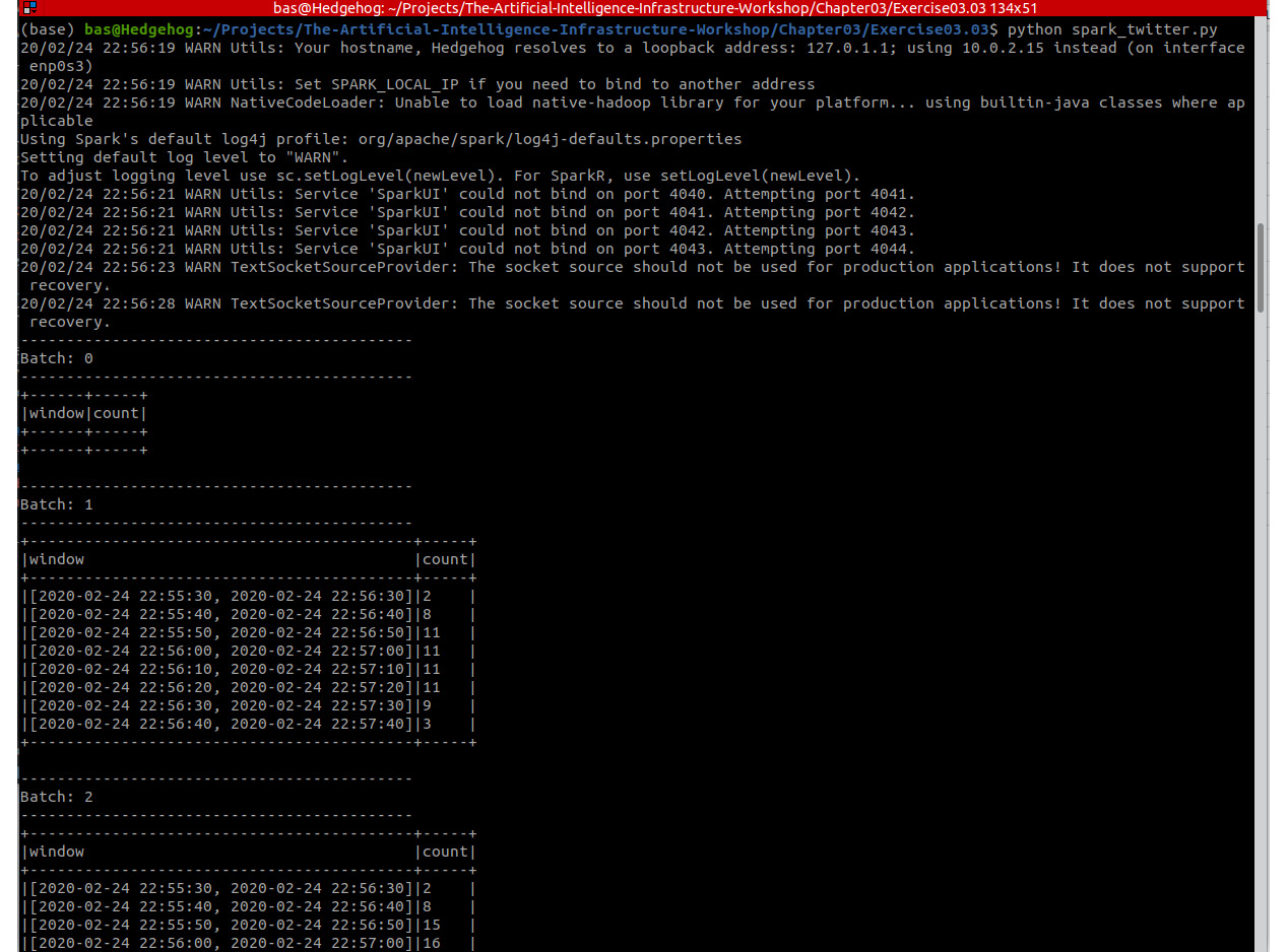
Figure 3.21: Output for the spark_twitter.py file
As you are experiencing now, your code runs in an infinite loop. The stream never ends. But, of course, the processing of the stream on your local machine can be stopped. To stop the stream processor, simply press Ctrl + C.
Note
To access the source code for this specific section, please refer to https://packt.live/2BYZEXE.
In this exercise, you have used Spark Structured Streaming to analyze a live Twitter feed. In the next activity, you'll continue to work with this framework to analyze the tweets and count the words in a certain time window.
Activity 3.02: Counting the Words in a Twitter Data Stream to Determine the Trending Topics
In this activity, you'll connect to Twitter in the same way as in Exercise 3.03, Streaming Data Processing with Spark. You can reuse the get_tweets.py or get_tweets.ipynb file that we have created. Only, this time, your goal is to group and count the words in the specified time window rather than the total amount of tweets. In this way, you can create an overview of the trending topics per time window.
Note
The code can be found here: https://packt.live/3iX0ODx.
Perform the following steps to complete the activity:
- Create a new Python file and name it spark_twitter.py.
- Write the Python code for the required imports and connect to a Spark cluster or a local instance with the SparkSession.builder object.
- Connect to the socket on the localhost and create the raw data stream by calling the readStream function of a SparkSession object.
- Convert the raw event strings from JSON to a useful format, namely a text field with the tweet text and a timestamp field that contains the event time. Do this by specifying the date-time format and the JSON schema and using the from_json PySpark function.
- Convert the field that contains the event time to a timestamp with the to_timestamp function.
- Split the text of the tweets into words by using the explode and split functions.
Hint: the tutorial of Spark Structured Streaming contains an example of how to do this.
- Create a tumbling window of 10 minutes with groupBy(window(…)). Make sure to group the tweets in two fields: the window, and the words of the tweets.
- Add a watermark that ensures that we have a slack of 1 minute before the window evaluates.
- Specify the evaluation function of the window: a count of all the words in the window.
- Send the output of the stream to the console and start executing the stream with the awaitTermination function.
You should get the following output:

Figure 3.22: Spark structured streaming job that connects to Twitter
Note
The solution to this activity can be found on page 592.
Summary
In this chapter, we have discussed many ways to prepare data for machine learning and other forms of AI. Raw data from source systems had to be transported across the data layers of a modern data lake, including a historical data archive, a set of (virtualized) analytics datasets, and a machine learning environment. There are several tools for creating such a data pipeline: simple scripts and traditional software, ETL tools, big data processing frameworks, and streaming data engines.
We have also introduced the concept of feature engineering. This is an important piece of work in any AI system, where data is prepared to be consumed by a machine learning model. Independent of the programming language and frameworks that are chosen for this, an AI team has to spend significant time writing the features and ensuring that the resulting code and binaries are well managed and deployed, together with the models themselves.
We have performed exercises and activities where we have worked with Bash scripts, Jupyter Notebooks, Spark, and finally, stream processing with live Twitter data.
In the next chapter, we will look into a less technical but very important topic for data engineering and machine learning: the ethics of AI.