Overview
This chapter introduces popular big data file formats and skims through their advantages and disadvantages. The file formats that are covered in the chapter are Avro, ORC, and Parquet. It will walk through the code snippets required to implement their transformation and conversion to the desired file format. It will also educate you on attributes such as compression and the read-write strategy and executing queries to highlight the operational performance.
By the end of the chapter, you will be able to select the optimum file format for any user-specific case. You will strengthen these concepts by applying them to a real-world situation and get first-hand experience of performing the necessary queries.
Introduction
In the previous chapter, we learned about SQL and NoSQL databases. Further, we introduced different databases, such as MySQL, MongoDB, and Cassandra, and implemented a hands-on experience to deal with real-world problems. Now we will extend our understanding of these databases and study the big data file formats.
Ever-growing competition in the industry has been reducing reaction times to nil and to keep up with this situation, businesses have to improvise their responses to the problems strategically. Businesses are continually facing challenges to improve the product offering, production, human resources, customer services, operations, and other facets of the business. To get a cutting edge over their competition, organizations have to apply many strategies, and analytics is one of the strategies that feeds on big data. A few companies that rely extensively on real-time big data applications are Facebook, Twitter, Apple, and Google.
Processing and analyzing this big data can become nasty within a short span with a snowball effect. To overcome it, data scientists and analysts have to put in place a reliable data storage strategy with the best of the tools available. We will discuss various attributes with which we can build the strong foundation needed to serve multiple business needs. We will begin by understanding the basic input file formats, after which we will learn about big data file formats such as Avro, Parquet, and ORC, along with their respective technical setups and format conversions.
We will be using Scala and Apache Spark for this course. Spark is a cluster-computing framework. It is an open-source tool. It can be used to process both batch and streaming data. The Scala programming language can be used for multiple application domains and so is a general-purpose language. Scala supports functional programming. It has a strong static type system where type checking occurs during compile time.
Let's begin by exploring the common file formats used for the exchange of data between systems. In the next section, we will cover the CSV and JSON file formats.
Common Input Files
Let's learn about the types of input files that are commonly used to exchange data between systems and the ways to convert them into various big data file formats. This section will also provide you with the programming skills required to transform these input files for the big data environment.
CSV – Comma-Separated Values
A CSV is a text file used to store tabular data separated by a comma. CSV is row-based data storage where each row is separated by a new line. For the exchange of tabular data, CSV files are frequently used.
The first row or header row of CSV files contains the schema detail, that is, column names for the data but not the type of data. CSV files fail to represent relational data, which means that a common column in multiple files does not have any relationship or hierarchy. Foreign keys are stored in columns of one or more files, but the CSV format itself does not express the linkage between these files.
The following figure is a screenshot of the Iris flower dataset, which contains data on three iris flower species. The dataset has 6 columns, namely, ID, SepalLengthCm, SepalWidthCm, PetalLengthCm, PetalWidthCm, and Species, and 150 rows. The Species column has a string value and the remaining four columns have rational numbers:

Figure 6.1: Comma-separated value format
The size of a CSV file can easily range from kilobytes (KBs) to gigabytes (GBs). Other reasons for the popularity of the CSV file format include the simplicity of the file structure and its portability.
JSON – JavaScript Object Notation
JSON (JavaScript Object Notation) data is a partially structured plain text file in which the data rests as key-value pairs. JSON can store data in a hierarchical format signifying the parent-child relationship between different pieces of data. JSON documents are small compared to other file formats of the same class, such as XML. The file size is the reason why it is preferred for network communication, notably in REST-based web services.
Various data processing applications support JSON serialization and deserialization. JSON documents can be converted or stored in highly performance-optimized files, but JSON works as raw data and can be used for the transformation of data.
The following figure is a screenshot of a JSON file:
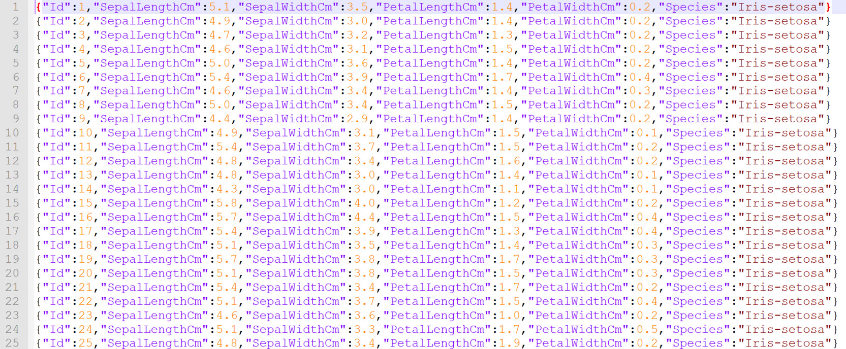
Figure 6.2: JavaScript Object Notation format
The size of JSON can vary from between a couple of megabytes (MBs) to tens of GBs. However, the JSON file format can support complex schema and occupy a larger memory space when compared to the CSV file format.
Now that we've learned about common input file formats, let's learn about the attributes based on which you can evaluate and select the appropriate big data file format for your application.
Choosing the Right Format for Your Data
In an environment where the data grows exponentially, it can take only days to reach terabytes (TBs), and in weeks, it can turn into petabytes (PBs). By then, it is not very easy to alter the chosen file format. Let's consider that a gaming company launches a multiplayer game every week, which generates a log of all the users' activities. The log size may grow exponentially for each game, depending on the number of users. So, selecting the appropriate big data file format is a challenging task.
Let's define the framework to evaluate different file formats and apply these attributes to the specific use case. This framework will not provide a directive approach. Nonetheless, it will attempt to be as far-reaching as possible.
Let's consider the basic framework for the selection of the format.
Selection Criteria:
- Orientation: row-based or column-based
- Partitions
- Schema evolution
- Compression
Orientation – Row-Based or Column-Based
Orientation is one of the most crucial factors to consider when selecting a big data format. It explains how data is stored inside the file. There are primarily two ways of storing data on the physical drive. Based on the usage of the application, you can select the file type. The columnar-based format can result in faster processing when performing analytical queries over a subset of the columns. For example, when we have to apply a sum function to a column, in that case, the values of all the cells in the rows that form a single column need to be processed.
Whereas, when we have to scan through all or the majority of the columns, then the row-based format can turn out to be effective. For example, imagine that you have to retrieve a user profile; in that case, the values of all the columns from a single row are required to be processed.
Let's examine these two types by extending this concept using the COVID-19 dataset, considering the following subset:

Figure 6.3: COVID 19 dataset
Row-Based
In the row-based format, all the columns of the rows are stored consecutively and retrieved one row at a time for processing. Row-based storage is highly efficient for transaction processing, which means that working with data involves interaction with all the columns over a group or all of the rows. In this orientation, writes of the data are very time-efficient.
When the previous table data is stored in the row-based format, it looks as follows:

Figure 6.4: Data storage structure in the row-based format
Column-Based
In the columnar-based format, the data in a column is stored sequentially, that is, from the first row to the last row, and while retrieving the data, only selected columns can be processed. The column-based format is very performant when working with analytical query models that require only a subset of columns from large datasets. In such cases, using row-based orientation will lead to a need for a lot of memory, which is resource-expensive and doesn't perform satisfactorily.
Saving the file in the column-based format stores the same data type (that is, column data) in adjacent physical space on the disk, impacting the I/O performance. In the columnar-based format, the query for applying various analytical functions over a column is efficient because the data in a single column can be extracted quickly, so it can be productive when applying functions over a few columns of data.
When the previous table data is stored in the column-based format, it looks as follows:

Figure 6.5: Data storage structure in the column-based format
The questions you need to ask when choosing the orientation are as follows:
- Do you require more reads or writes?
Try to identify the intent of the application, and consider whether the usage of the application will lead to more read commands, indicating a need for a data retrieval system, or more write commands, indicating a need for a data acquisition system.
- Does your application have a transactional or analytical approach?
For this question, you need to envision the volume of interaction with the data. For example, the user log for a multiplayer game will be analytically queried about first-time logins or how much time is spent on each level, and so on. These queries are applied across a single column.
On the contrary, the gamer's profile will interact with the data limited to a single row. The gamer's profile may have attributes including name, age, level, batches, and so on. These attributes will be updated and retrieved in a predictable pattern accessing a single row from a table or only a few rows from multiple tables.
Let's learn about another important attribute, namely, partitions.
Partitions
In a big data environment, processing data is challenging primarily because of the size of the files. These files have to be processed in chunks or small parts, which can be achieved with file partitioning. These splits are done as per the Hadoop Distributed File System (HDFS) block and impact the processing time.
The chunk that is created can be loaded in memory to be processed individually. The ability to partition the data and process it independently is the foundation of the scalable parallelization of processing. The parallel processing capability of the file is the key to its selection.
Let's learn about another important attribute, namely, schema evolution.
Schema Evolution
Choosing the optimum file format cannot be completed until schema evolution has been considered. In the case of continuous streaming data, the schema is bound to be changed over time and, most importantly, multiple times. The schema includes columns, data types, views, primary keys, relationships, and more.
Very rarely, it will happen that the schema present at the time of creating the file is perpetual. For other instances where the transition between the old schema and a new schema is required, a file format should have the provision to adopt these changes smoothly, such as if a gaming company decides to start a daily championship, which means that an additional leaderboard is required. This will require schema evolution.
There are a few questions to answer, without which your consideration of changing the schema will not be complete:
- Will there be difficulties in adopting the new schema?
- What is the impact on the disk storage of the file?
- Will there be compatibility issues between different versions?
We will be covering these questions with regard to each file type that we cover. Let's learn about another important attribute, namely, compression.
Compression
Data compression is a necessary evil that decreases the amount of data to be stored or transmitted. It helps in optimizing the use of time and money by shrinking data that otherwise would have used more space. It reduces the size of the file to be stored on the disk and speeds up data exchange throughout the network. This is attempted at the source of the data by using encoding on repeated data, which can result in a great reduction in size. A few encoding types are as follows:
- Dictionary encoding
- Plain encoding
- Delta encoding
- Bit-packing hybrid
- Delta-length byte array
- Delta strings (incremental encoding)
For illustration, let's look at dictionary encoding and consider the Species column from the Iris dataset.
Dictionary Encoding: This is a type of data compression technique that works by mapping the actual data to a token/symbol ("dictionary"). The tokens/symbols are smaller than the actual data, resulting in compression.
The unique values from the Species column are associated with corresponding values, and the dictionary will be stored separately. The new value will be stored in the file with other data, which is converted as follows:

Figure 6.6: Dictionary encoding
It will create a dictionary of all the unique values from a column and link them to a corresponding unique value. This step reduces the storage of repeated values in a column, and overall reduces demand for storage space and the transmission of the data.
These attributes will provide a foundation based on which you can evaluate the file format and select the most suitable file format for your application. Let's learn about the various file formats in the next section.
Introduction to File Formats
Now, let's understand the file structure in detail and distinguish between these file formats. This section will decompose the file formats and dive into the structure of files to elaborate on the efficiency of each file format.
Parquet
Apache Parquet is an open-source column-oriented representation and stores data in an optimized columnar format. It is language-independent and framework-independent because the objective of creating this format was to optimize the operation and storage of data across Hadoop.
Shortly after its introduction, it acquired popularity in the industry. The reasons for its acceptance are primarily the fast retrieval and processing capabilities that it offers. However, writes are usually time-consuming and considerably expensive.
As it is a columnar-based format, homogenous data is stored together, resulting in better compression. The compression and encoding scheme can have a significant impact on performance.
Let's explore the elements of the Parquet file format and consider the following figure:

Figure 6.7: Parquet file structure
Parquet has nested data structures stored in a columnar-based format. A file can be decomposed into the following elements.
Firstly, the header, which is the apex of the file that contains the magic number (PAR1), communicating that the file type is PARQUET to the application.

Figure 6.8: Parquet file structure
The second part is the data block, which is composed of the row groups, meaning a chunk of the actual data or a subset of the total number of rows. Each row group has multiple instances of column data that contains data pages for different chunks of column data. The page contains the metadata, repetition level, definition level, and the encoded column data. The metadata contains details about the chunk of column data, such as min, max, and count. The default value of the row group is 128 MB.
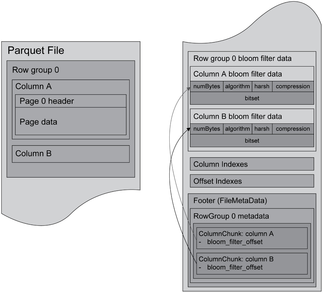
Figure 6.9: Parquet file structure
The last is the Footer, which includes the format version, the schema details, and the metadata of the columns in the file. It also includes an attribute for the footer length encoded as a 4-byte field, terminated by a 4-byte magic number (PAR1), the same as the header.
Let's now learn about partitioning and compression in the Parquet file format.
Partitioning and Compression
The ability to partition Parquet files makes them a superior selection, and their columnar structure enables a comparatively faster scan than other file formats. The compression contributes to another significant attribute, which is that Parquet compression can significantly reduce the size. Therefore, the compression helps in enhancing performance, data ingestion, and data access.
Let's now learn about schema evolution for the Parquet file format.
Schema Evolution
Over the life of the application, there will be a need to alter the schema, and the incessant data flow may turn this into a nightmare. You can evolve the schema, which means adding new columns as and when needed. The schema evolution generates different Parquet files but they are mutually compatible schemas.
Platform Support
While taking a final decision on which file format is most suitable, taking into account the harmony between the file format and the platform is an important consideration. Spark has comprehensive support for the Parquet file format. Let's now look at a synopsis of the Parquet file format:

Figure 6.10: Parquet attributes synopsis
The synopsis assesses the performance of each attribute of the Parquet file format and draws conclusions as a visually comparable scale. Parquet files perform moderately in schema evolution and above-moderately in attributes such as partitioning and compression.
Now we will proceed to the next exercise and create a Parquet file from common input file formats.
Exercise 6.01: Converting CSV and JSON Files into the Parquet Format
To start with a big data environment, you are required to import data into the environment. Usually, this data is available in CSV or JSON formats. This exercise aims to use a dataset in two input formats, that is, CSV and JSON files, and convert them into Parquet format. After converting the CSV file, we will read and display the contents of the output Parquet file to validate the conversion.
We will be working with a dataset containing census data that consists of 6 columns and 1,321,975 rows, taken from the New Zealand government's stats website (https://www.stats.govt.nz/large-datasets/csv-files-for-download/). The columns are Year, Age, Ethnic, Sex, Area, and count. This dataset is available in the CSV file format (41 MBs) and the JSON file format (106 MBs). The size difference is because the CSV file is compact, primarily due to its simpler schema structure. The dataset has some null values present as well.
The dataset can be found in our GitHub repository at the following location:
You need to download and extract the Census_csv.rar and Census_json.rar files from the GitHub repository.
Before proceeding to the exercise, we need to set up a big data environment by installing Scala and Spark. Please follow the instructions in the Preface to install it.
Perform the following steps to complete the exercise:
- Create a directory called Chapter06 for all the exercises and activities of this chapter. In the Chapter06 directory, create the Exercise06.01 and Data directories to store the files for this exercise.
- Move the extracted CSV and JSON files to the Chapter06/Data directory.
- Open your Terminal (macOS or Linux) or Command Prompt window (Windows), move to the installation directory, and open the Spark shell in it using the following command:
spark-shell
You should get the following output:

Figure 6.11: Spark shell
- Read the CSV file using the following code:
var df_census_csv = spark.read.options(Map("inferSchema"- >"true","delimiter"->",","header"- >"true")).csv("F:/Chapter06/Data/Census.csv")
Note
Update the input path of the file according to your local file path throughout the exercises in this chapter.
You should get the following output:
df_census_csv: org.apache.spark.sql.DataFrame = [Year: int,
Age: int … 4 more fields]
This command creates a DataFrame variable (df_census_csv) and loads the contents of the CSV file into the variable.
- Read the JSON file using the following code:
var df_census_json = spark.read.json(
"F:/Chapter06/Data/Census.json")
Note
Owing to the size of the data, the commands in this exercise can take up to a few minutes to execute.
You should get the following output:
df_census_json: org.apache.spark.sql.DataFrame = [Age: bigint,
Area: string … 4 more fields]
- Show the CSV file using the following command:
df_census_csv.show()
You should get the following output:
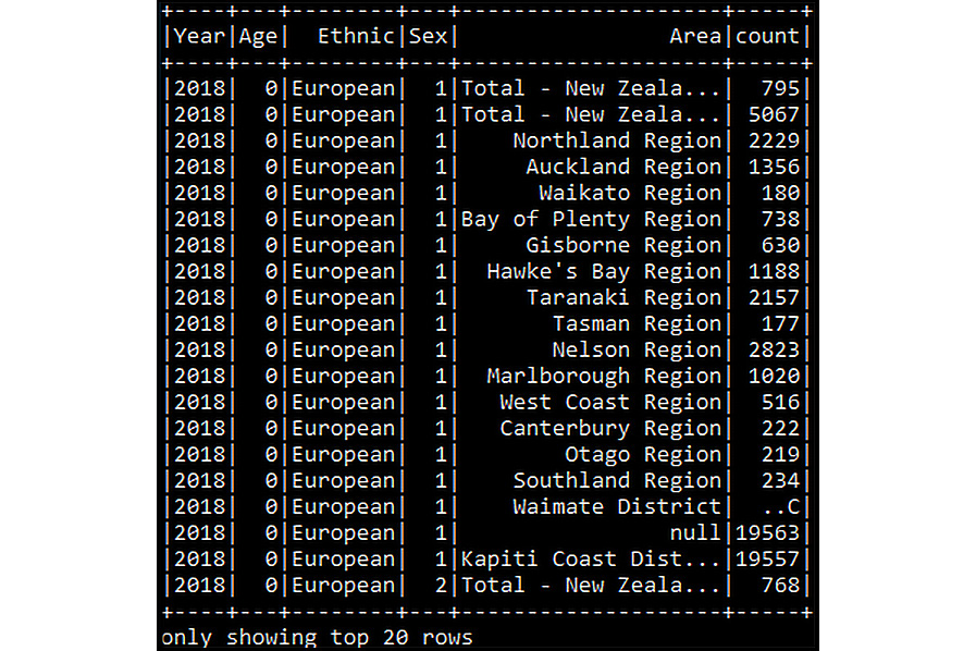
Figure 6.12: Displaying the CSV DataFrame
This command will display the first 20 rows of the DataFrame created in the previous step.
- Show the JSON file using the following command:
df_census_json.show()
You should get the following output:
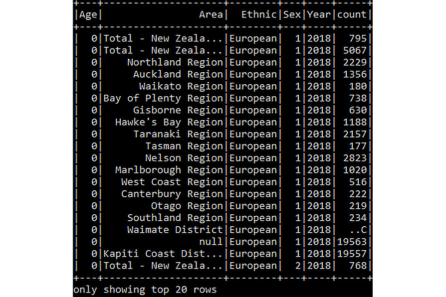
Figure 6.13: Displaying the JSON DataFrame
This command will display the first 20 rows of the DataFrame created in the previous step.
- Convert the Census.csv file to the Parquet format using the following code:
df_census_csv.write.parquet(
"F:/Chapter06/Data/Output/census_csv.parquet")
A file is created of the following size:
Output file size: 16.6 MB
This command will write the CSV DataFrame into the Parquet file format. The first argument is the path of the output file.
- Convert the Census.json file to the Parquet format using the following code:
df_census_json.write.parquet(
"F:/Chapter06/Data/Output/census_json.parquet")
A file is created of the following size:
Output file size: 1.18 MB
This command will write the JSON DataFrame into the Parquet file format. The function argument is the path of the output file.
- Verify the saved file using the following code:
val df_census_parquet = spark.read.parquet(
"F:/Chapter06/Data/Output/census_csv.parquet")
You should get the following output:
df_census_parquet: org.apache.spark.sql.DataFrame = [Year: int,
Age: int … 4 more fields]
This command will create a DataFrame (df_census_parquet) and load the Parquet file content into the DataFrame.
- Open the Parquet file using the following code:
df_census_parquet.show()
You should get the following output:
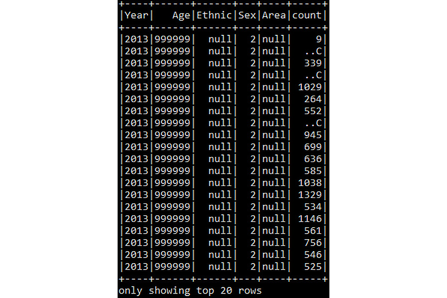
Figure 6.14: Displaying the Parquet DataFrame
This command will display the first 20 rows of the DataFrame created in the previous step.
Note
Similarly, the output Parquet file from the JSON DataFrame can be loaded and verified.
Note
To access the source code for this specific section, please refer to https://packt.live/32eGNT8.
By completing the exercise, you will be able to create a DataFrame and load data from CSV and JSON files into it. You will also be able to convert the created DataFrame into the Parquet file format and load the Parquet file in a new DataFrame. Let's learn about the Avro file format in the next section.
Avro
Avro is a row-based file format that can be partitioned easily. It is a language-independent data serialization system that can be processed in multiple programming languages. The schema, which is saved as JSON format, is associated separately with the read and write operations. However, the actual data is converted to a binary format, resulting in reduced file size and improved efficiency.
The serialization converts the data into a highly compact binary format, which any application can deserialize.
It has a reliable provision for schema evolution that adds new fields or changes the existing fields. This feature makes the older file version compatible with the existing code with the least amount of modification.
Because the schema is written in JSON format, this makes it more comprehensive to understand the fields and their data types. In a big data environment, Avro is usually the first preference due to the extremely efficient write capability in a hefty workload.
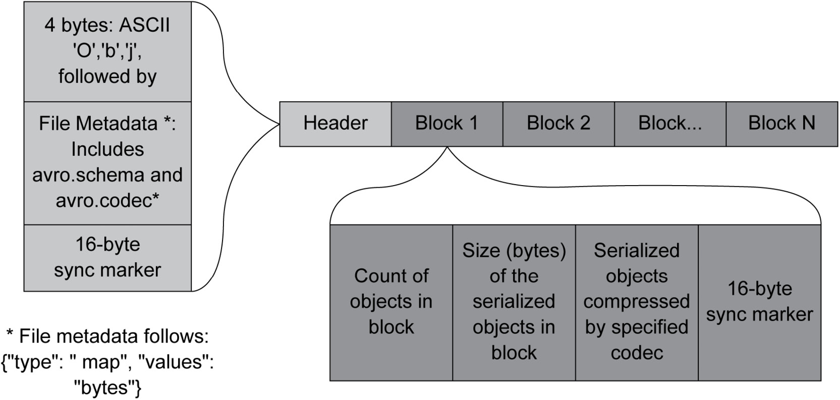
Figure 6.15: Avro file structure
The file structure of the Avro file contains a header and a data block. The header contains a 4-byte string, 'O', 'b', 'j', and file metadata. The data block is comprised of the count of the object in the block, a size 16-byte sync marker, and the serialized object of the actual data.
Platform Support
While making a final decision on which file format is most suitable, taking into account the potential harmony with the platform is an important consideration. The Avro file format works optimally with Kafka. Let's now look at a synopsis of the Avro file format:

Figure 6.16: Avro attribute synopsis
The synopsis assesses the Avro format's efficiency with regard to various attributes. The Avro file format performs moderately on compression, above-moderately on partitioning, and performs very well in the case of schema evolution.
Now we will proceed to the next exercise and create an Avro file from common input file formats.
Exercise 6.02: Converting CSV and JSON Files into the Avro Format
This exercise aims to use a dataset in both input formats, that is, CSV and JSON files, and convert it into the Avro format, which is another big data file format. We will use the same dataset from Exercise 6.01, Converting CSV and JSON Files into the Parquet Format. After converting the CSV file, we will read and display the content of the output Avro file to validate the conversion.
Perform the following steps to complete the exercise:
- In the Chapter06 directory, create an Exercise06.02 directory to store the files for this exercise.
- Open your Terminal (macOS or Linux) or Command Prompt window (Windows), move to the installation directory, and open the Spark shell in it using the following command:
spark-shell --packages org.apache.spark:spark-avro_2.11:2.4.5
Note
The spark-avro packages are not included by default and to launch the Spark shell with the spark-avro dependency, we will use the –packages argument.
You should get the following output:

Figure 6.17: Spark shell
- Read the CSV file using the following code:
var df_census_csv = spark.read.options(Map(
"inferSchema"->"true","delimiter"->",","header"->"true")
.csv("F:/Chapter06/Data/Census.csv")
Note
Update the input path of the file according to your local file path throughout the exercise.
You should get the following output:
df_census_csv: org.apache.spark.sql.DataFrame = [Year: int,
Age: int … 4 more fields]
This command creates a DataFrame variable (df_census_csv) and loads the contents of the CSV file into the variable.
- Read the JSON file using the following code:
var df_census_json = spark.read.json("F:/Chapter06/Data/Census.json")
Note
Owing to the size of the data, the commands in this exercise can take up to a few minutes to execute.
You should get the following output:
df_census_json: org.apache.spark.sql.DataFrame = [Age: bigint,
Area: string … 4 more fields]
- Show the CSV file using the following command:
df_census_csv.show()
You should get the following output:
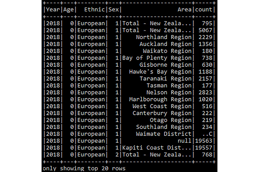
Figure 6.18: Displaying the CSV DataFrame
This command will display the first 20 rows of the DataFrame created in the previous step.
- Show the JSON file using the following command:
df_census_json.show()
You should get the following output:
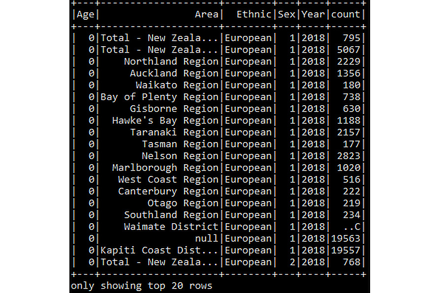
Figure 6.19: Displaying the JSON DataFrame
This command will display the first 20 rows of the DataFrame created in the previous step.
- Convert the Census.csv file to the Avro format using the following code:
df_census_csv.write.format("avro").save(
"F:/Chapter06/Data/Output/census_csv.avro")
A file is created of the following size:
Output file size: 70.8 MB
This command will write the CSV DataFrame into the Avro file format. The first argument is the path of the output file.
- Convert the Census.json file to Avro format using the following code:
df_census_json.write.format("avro")
.save("F:/Chapter06/Data/Output/census_json.avro")
A file is created of the following size:
Output file size: 5.0 MB
This command will write the JSON DataFrame into the Avro file format. The function argument is the path of the output file.
- Verify the saved file using the following code:
var df_census_avro = spark.read.format("avro").load(
"F:/Chapter06/Data/Output/census_csv.avro")
You should get the following output:
df_census_avro: org.apache.spark.sql.DataFrame = [Year: int,
Age: int … 4 more fields]
This command will create a DataFrame (df_census_avro) and load the Avro file content into the DataFrame.
- Open the Avro file using the following code:
df_census_avro.show()
You should get the following output:

Figure 6.20: Displaying the Avro DataFrame
This command will display the first 20 rows of the DataFrame created in the previous step.
Note
To access the source code for this specific section, please refer to https://packt.live/32boIFh.
By completing this exercise, you are now able to create a DataFrame and load the data from CSV and JSON files. You are also able to convert the created DataFrame into the Avro file format and also load the Avro file in a new DataFrame. Let's learn about the ORC file format in the next section.
ORC
Apache ORC (an abbreviation for Optimized Row Columnar) is a column-oriented data format available in the Apache Hadoop environment. You can conceive the structure of an ORC file as divided into three sub-parts, which are Header, Body, and Footer, as shown in the following figure:

Figure 6.21: ORC file structure
The header is comprised of the keyword ORC in case the application requires a determination of the file type while processing.
The body holds the transaction data and indexes, and the transaction data is saved in row chunks known as stripes. The default stripe size is 250 MB, however, increasing the stripe size can increase the read efficiency at the cost of memory.
Each stripe is further apportioned into three sections, that is, the actual data sandwiched between an index section on top and a stripe footer section.
The stripe index holds quick aggregations of the actual data, such as the max and min values, and its row index within that column. The index saves the information required to determine the stripe matching the data needed and the section of the row. The stripe footer includes the encoding information of the columns and the stream directory with its location.
The footer segment is comprised of the layout of the body of the file, statistics about each column, and schema information. It is constructed from three sub-parts, mainly the footer, which is topped by metadata and postscript segments. The metadata segment comprises the statistical information describing columns stored at the stripe level. The file footer has data related to the list of stripes, the number of rows per stripe, and the data type of the column. It has aggregate values for columns, such as min, max, and sum. The postscript segment gives the file information, such as the extent of the file's footer and metadata sections, the file version, and the compression parameters.
Platform Support
When taking a final decision on which file format is most suitable, taking into account the compatibility with the platform is an important consideration. The ORC file format works optimally with Hive since this file format was made for Hive.
Let's now look at a synopsis of the ORC file format:

Figure 6.22: ORC attribute synopsis
The synopsis summarizes the performance of the ORC file format with regard to various attributes. The ORC file format is not compatible with schema evolution but works well for applications that require the functionalities of partitioning and compression.
Now we will proceed to the next exercise and create an ORC file from common input file formats.
Exercise 6.03: Converting CSV and JSON Files into the ORC Format
This exercise uses a dataset in both input formats, that is, CSV and JSON files, and converts it into the ORC format. We will use the same dataset from Exercise 6.01, Converting CSV and JSON Files into the Parquet Format. After converting the CSV file, we will read and display the contents of the output Parquet file to validate the conversion.
Perform the following steps to complete the exercise:
- In the Chapter06 directory, create the Exercise06.03 directory to store the files for this exercise.
- Open your Terminal (macOS or Linux) or Command Prompt window (Windows), move to the installation directory, and open the Spark shell in it using the following command:
spark-shell
You should get the following output:

Figure 6.23: Spark shell
- Read the CSV file using the following code:
var df_census_csv = spark.read.options(Map(
"inferSchema"->"true","delimiter"->",","header"->"true"))
.csv("F:/Chapter06/Data/Census.csv")
Note
Update the input path of the file according to your local file path throughout the exercise.
You should get the following output:
df_census_csv: org.apache.spark.sql.DataFrame = [Year: int,
Age: int … 4 more fields]
This command creates a DataFrame variable (df_census_csv) and loads the contents of the CSV file into the variable.
- Read the JSON file using the following code:
var df_census_json = spark.read.json(
"F:/Chapter06/Data/Census.json")
Note
Owing to the size of the data, the commands in this exercise can take up to a few minutes to execute.
You should get the following output:
df_census_json: org.apache.spark.sql.DataFrame =
[Age: bigint, Area: string … 4 more fields]
- Show the CSV file using the following command:
df_census_csv.show()
You should get the following output:

Figure 6.24: Displaying the CSV DataFrame
This command will display the first 20 rows of the DataFrame created in the previous step.
- Show the JSON file using the following command:
df_census_json.show()
You should get the following output:

Figure 6.25: Displaying the JSON DataFrame
This command will display the first 20 rows of the DataFrame created in the previous step.
- Convert the Census.csv file to the ORC format using the following code:
df_census_csv.write.orc(
"F:/Chapter06/Output/census_csv.orc")
A file is created of the following size:
Output file size: 16.5 MB
This command will write the CSV DataFrame into the ORC file format. The first argument is the path of the output file.
- Convert the Census.json file to the ORC format using the following code:
df_census_json.write.orc(
"F:/Chapter06/Output/census_json.orc")
A file is created of the following size:
Output file size: 1.1 MB
This command will write the JSON DataFrame into the ORC file format. The function argument is the path of the output file.
- Verify the saved file using the following code:
val df_census_orc = spark.read.orc("F:/Chapter06/Data/Output/census_csv.orc")
You should get the following output:
df_census_orc: org.apache.spark.sql.DataFrame = [Year: int, Age: int … 4 more fields]
This command will create a DataFrame (df_census_orc) and load the ORC file contents into the DataFrame.
- Open the ORC file using the following code:
df_census_orc.show()
You should get the following output:

Figure 6.26: Displaying the ORC DataFrame
This command will display the first 20 rows of the DataFrame created in the previous step.
Note
To access the source code for this specific section, please refer to https://packt.live/309p10I.
By completing the exercise, you will be able to create a DataFrame and load the data from CSV and JSON files. You will also be able to convert the created DataFrame into the ORC file format and load the ORC file in a new DataFrame.
We can observe that the conversions to each file format have resulted in different file sizes owing to the different compression algorithms, schemas, and a few other attributes. Your selection, however, should not just depend upon the size alone but also on the performance of the query execution.
We will now move on to query performance, where we will learn how we can measure the performance of queries on these file formats.
Query Performance
So far, we have learned how to convert an input file, create DataFrames, and load big data files into these DataFrames. Now, on these DataFrames, we will execute different types of queries to measure the execution performance. To measure the performance, we will create a time function, which will return the time required to execute a query.
The code of the function to do this is as follows:
# Function to measure time for query execution
def time[A](f: => A) = {
val s = System.nanoTime
val ret = f
println("Time: "+(System.nanoTime-s)/1e6+" ms")
ret
}
This function, named Time, takes an input argument denoted by A and then executes the query provided in the argument.
Note
The function will result in the output and print the time taken for execution in milliseconds.
Now let's look at the different types of queries that we will execute to measure performance. There are two methods to execute a query over a dataset. The first is to execute queries directly to the DataFrame, and the second is to create a view and run SQL commands over that view. The latter provides the infrastructure to execute complex queries. Let's look into both of these methods.
Method One: DataFrame Operations
In this method, we will use DataFrame functions to query the DataFrame:
\ Define spark dataframe
var dataframe = spark.read.json("F:/Chapter06/Data/Census.json")
\ This will count the number of records (rows)
\from the dataframe
dataframe.count()
\ We can time the query using the time function create above.
time{dataframe.count()}
More functions can be found on Apache's website, at https://spark.apache.org/docs/2.2.0/api/scala/index.html#org.apache.spark.sql.functions$.
Method Two: Global Temporary View
- Create a view from the DataFrame:
dataframe.createOrReplaceTempView("view_name")
Here, we create a view from the DataFrame by using createOrReplaceTempView. It creates or replaces the view name provided to it. The view will be created in Spark's default database and it can be used like a table in Spark SQL. It is session-scoped, which means it will be destroyed after the session is terminated.
- Formulate the query and use the spark.sql() function to execute the query:
\ Defining sql query as a variable
val sql_query = "Select count(*) from view_name"
\ We can time the query using the time
\function create above.
time{spark.sql(sql_query)}
The SQL function in SparkSession facilitates applications to execute SQL queries and returns the result as a DataFrame.
We will move on to the next activity, where we will consider a real-world scenario and apply what we've learned from this chapter.
Activity 6.01: Selecting an Appropriate Big Data File Format for Game Logs
This activity focuses on selecting the most suitable big data format from the different file formats available. The selection will be based on size, performance, and current technology to provide the best solution for the given requirements.
You have been recently hired as a data engineer by gaming company XYZ, located in Seattle. They specialize in developing popular and intriguing war games for multiple online users. This results in millions of log records being generated each day, consuming high amounts of storage on the cloud. The trend of the log size and its increasing storage consumption is a concern for the company, and they are determined to resolve this by looking at the various big data file formats available.
The log data comes in JSON format composed of the following columns: user_id, event_date, event_time, level__id, and session_nb. The company is already utilizing the capabilities of Cloudera and Spark as a part of the big data technology stack.
The analytics team requires the data to be of the smallest size possible that will maintain the operational performance for analytical queries. As a data engineer, the company expects you to analyze and suggest the best file format for this use case, supporting your suggestion with appropriate findings. The decision does not hinge only on compressed file sizes, but on several other factors, so we will store this data in all the file formats that we learned about earlier and perform an operation to find the best-suited format among them for our requirements.
We will be using a sample dataset that was created by the author. The dataset can be found in our GitHub repository at the following location: https://packt.live/2C72sBN.
You need to download the session_log.rar file from the GitHub repository. After unzipping it, you will have the session_log.csv file.
Note
The code for this activity can be found at https://packt.live/2OhITcH.
Perform the following steps to complete the activity:
- Load the data from the CSV file.
- Show the data to verify the load command.
- Convert the input file into the Parquet, Avro, and ORC file formats and verify the file size of each.
- Create a function for query performance.
- Perform and measure the time taken for query execution over each file format for count and GROUP BY queries.
- Find the file with the highest compression and quickest query response.
- Conclude which is the most feasible file format based on the current technology of the company.
Note
The solution to this activity can be found on page 616.
Summary
In this chapter, we have learned about common input file formats for big data, such as CSV and JSON. We also learned about popular file formats, namely Parquet, Avro, and ORC, which are useful in the big data environment and looked at essential decision points for making a choice on which to use. We explored the conversion to each of these file formats from the CSV and JSON formats and executed them in a big data environment using Spark and Scala. To strengthen the concept, we executed each format conversion in the respective exercises.
At the end of the chapter, we looked at a real-world business problem and concluded which was the most suitable file format based on the selection criteria learned in this chapter.
In the next chapter, we will extensively cover the vital infrastructure of the big data environment known as Spark. This will lay a strong foundation of the concept and also lead us through the journey of creating our first pipeline in Spark.