Chapter 4: Format and Memory Handling

I've continuously extolled the virtues of using Arrow as a data interchange technology for tabular data, but how does it stack up against the more common technologies that people tend to utilize for transferring data? When does it make sense to use one over the other for your application programming interface (API)? The answer is to know how different technologies utilize memory. Clever management of your memory can be the key to performant processes. To decide which format to use for your data, you need to understand which use cases your options were designed for. With that in mind, you can take advantage of the runtime properties of the most common data transport formats such as Protocol Buffers (Protobuf), JavaScript Object Notation (JSON), and FlatBuffers when appropriate. By understanding how to utilize memory in your program, you can process very large amounts of data with minimal memory overhead.

We're going to cover the following things in this chapter:

• Which use cases make sense for using Arrow versus using Protobuf, JSON, FlatBuffers, or storage formats such as comma-separated values (CSV) and Apache Parquet
• Processing huge 100-gigabyte (GB) files using only a few megabytes (MB) of physical random-access memory (RAM) by utilizing memory mapping

Technical requirements

As before, you'll need an internet-connected computer with the following software so that you can follow along with the code examples here:

• Python 3.7 or higher, with the pyarrow and pandas modules installed
• Go 1.16 or higher
• A C++ compiler capable of compiling C++11 or higher, with the Arrow libraries installed
• Your preferred IDE, such as Emacs, Sublime, or VS Code
• A web browser

Storage versus runtime in-memory versus message-passing formats

When we're talking about formats for representing data, there are a few different, complementary, yet competing things we typically are trying to optimize. We can generally (over-) simplify this by talking about three main components, as follows:

• Size—The final size of the data representation
• Serialize/deserialize speed—The performance for converting data between the formats and something that can be used in-memory for computations
• Ease of use—A catch-all category regarding readability, compatibility, features, and so on

How we choose to optimize between these components is usually going to be heavily dependent upon the use case for that format. When it comes to working with data, there are three high-level use case descriptions I tend to group most situations into: long-term storage, in-memory runtime processing, and message passing. Yes—these groupings are quite broad, but I find that every usage of data can ultimately be placed into one of these three groups.

Long-term storage formats

What makes a good storage format? Size is typically considered first, as you're often sharing files and storing large datasets in a single format. With the advent and proliferation of cloud storage, storage costs aren't the driving reason for this so much as input-output (I/O) costs. You can use Amazon's Simple Storage Service (S3) storage or Microsoft's Azure Blob Storage and get nearly limitless storage for pennies or better, but when you want to retrieve that data, you're going to pay in bandwidth costs and network latency if the data is very large.

Depending on the way the data is going to be used, you're also going to be often trading off between optimizing for reads and optimizing for writes, as optimizing for one is usually going to be sub-optimal for the other. Some examples of persistent storage formats are provided here:

• CSV
• Apache Parquet
• Avro
• Optimized Row Columnar (ORC)
• JSON

In almost all cases, binary formats are going to be smaller and more efficient than plain text formats simply by virtue of the ability to represent more data with fewer bytes. You just have to sacrifice some of that ease of use since we can't just read binary data with our eyes! Unless you're a robot… Anyway, this is why most of the time, it is recommended for data to be stored in compact binary formats such as Parquet instead of text formats such as CSV or JSON. When we're looking at data stored on disk, there are two ways to optimize for reads, as outlined here:

• Make the physical size of the data smaller
• Use a format that minimizes how much data needs to be read to satisfy a query

Because reading from a disk—even solid-state disks (SSDs)—is so much slower than reading from memory, the bottleneck for processing will be how much data needs to be read into memory to get the data needed. While this can make it very efficient to read the data from disk into the main memory, it still requires decompressing that data before you can work with it, making it less optimal for being an in-memory computational format, as shown in the following diagram:

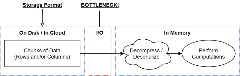
Figure 4.1 – Workflow to bring stored data into memory

Binary formats are often easier to compress based on how they store the data and can sometimes use tricks to make the data even more compressible. Parquet and ORC store the data in column-oriented forms that are generally more compressible than CSV and Avro, for example. You also have to take into account the way the data will be used. While you might be able to get a smaller file size with column-oriented storage formats, this is most beneficial if your most common workflow is to only need a subset of columns from the rows. The most common workflows for modern big data are online transaction processing (OLTP) and online analytical processing (OLAP).

OLTP systems usually process data at a record (row) level and perform Create, Read, Update, Delete (CRUD) operations on each record as a whole. The tasks performed by an OLTP system are focused on maintaining the integrity of the data when being accessed by multiple users at once and measuring their effectiveness by the number of transactions per second they can process. In the vast majority of cases, an OLTP system will want the entire record of data, not just a subset of fields. For this type of workflow, a row-based storage format such as Apache Avro would be most beneficial since you're usually going to need entire rows anyway.

OLAP systems are designed to quickly perform analytical operations such as aggregations, filtering, and statistical analysis across multiple dimensions such as time or other fields. As mentioned in previous chapters, this type of workflow benefits more from column-oriented storage so that you can minimize I/O by only reading the columns of data you need and ignoring fields that are irrelevant to the query. By aligning data of the same type next to each other, you get higher compression ratios and can optimize the representation of null values in sparse columns.

Once you read data from a storage format, you're going to need to convert the data into a different representation in order to work with it and perform any computations you want on it. This representation is referred to as the in-memory runtime representation or format, as shown in the following diagram:

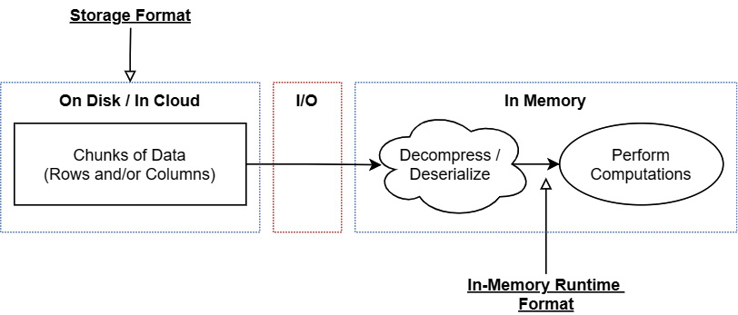
Figure 4.2 – Storage format and in-memory runtime

In the majority of cases, the I/O cost will be significantly larger than the cost to decompress or deserialize the data into a usable, in-memory representation, but this is still a cost that is proportional to the size of the data and needs to be paid before any operations can be performed. There are exceptions to this, of course. There do exist specific formats and algorithms that allow us to perform operations on compressed data without decompressing it, but they are typically uncommon and very specialized cases.

So, when we convert that data into some representation that we can perform operations on, which formats could we use? Well…

In-memory runtime formats

Formats such as Arrow and FlatBuffers have an inter-process representation that is identical to their in-memory representation, allowing developers to avoid the cost of copies when passing the data from one process to another, whether it's across a network or between processes on the same machine. The goal of formats that fall into this class is to be optimized for computation and calculation.

When working with the data in memory, the size of the data is less relevant than with on-disk formats. When performing computations and analysis in memory, the bottleneck is the central processing unit (CPU) itself rather than slow-moving I/O. In this situation, the major ways that modern developers speed up performance are through better algorithmic usage and optimizations such as vectorization. As such, data formats that can better take advantage of these end up being more performant for analytical computations. This is why Arrow is designed the way it is, optimizing for the most common analytical algorithms and taking advantage of single instruction, multiple data (SIMD) vectorization as opposed to optimizing for disk-resident data. You'll recall that we covered SIMD back in Chapter 1, Getting Started with Apache Arrow.

There are other concerns that can make a difference, such as byte alignment and random reads versus sequential reads, which can affect the performance of in-memory processing and disk-resident processing differently. Modern CPUs don't execute one instruction at a time but instead use a pipeline to stagger how instructions are executed through different stages. To maximize throughput, all kinds of predictions about which instructions will be next are made to keep the pipeline as full as possible. See the following screenshot for a simplified example of this pipeline concept:

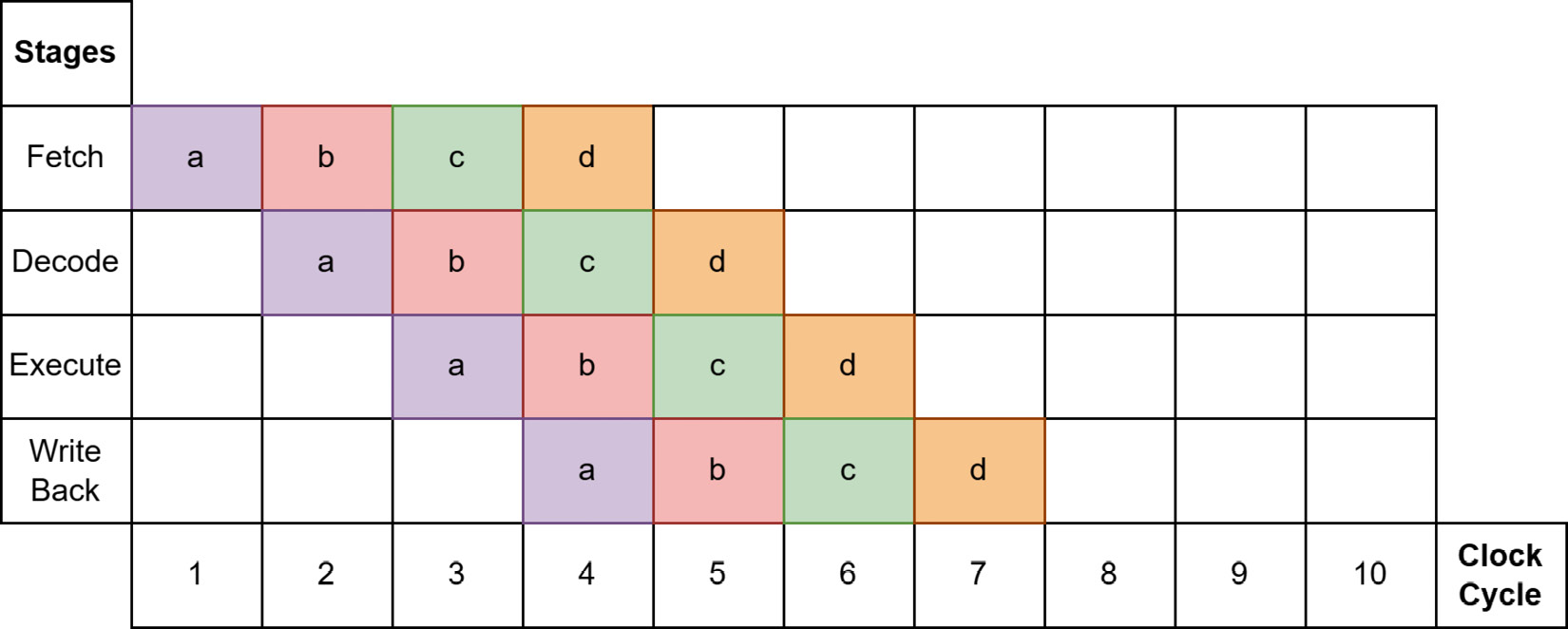
Figure 4.3 – Ideal pipeline case

As long as the processor's predictions are correct, everything keeps chugging along smoothly as fast as it can, and Figure 4.3 shows all four instructions completed in seven clock cycles. The hardware is going to try to predict which memory locations will be needed by the CPU and preload that data into registers before the instruction that needs it gets executed. As a result, sequential reads of contiguous chunks of memory can be extremely fast because the processor can make easy predictions and load larger chunks of data into the main memory with fewer instructions. The usage of vectorization by Arrow libraries also helps achieve this throughput, with instructions that are highly predictable for modern processors. Whenever the processor's prediction is incorrect, we get what's called a bubble, as seen in the following screenshot:

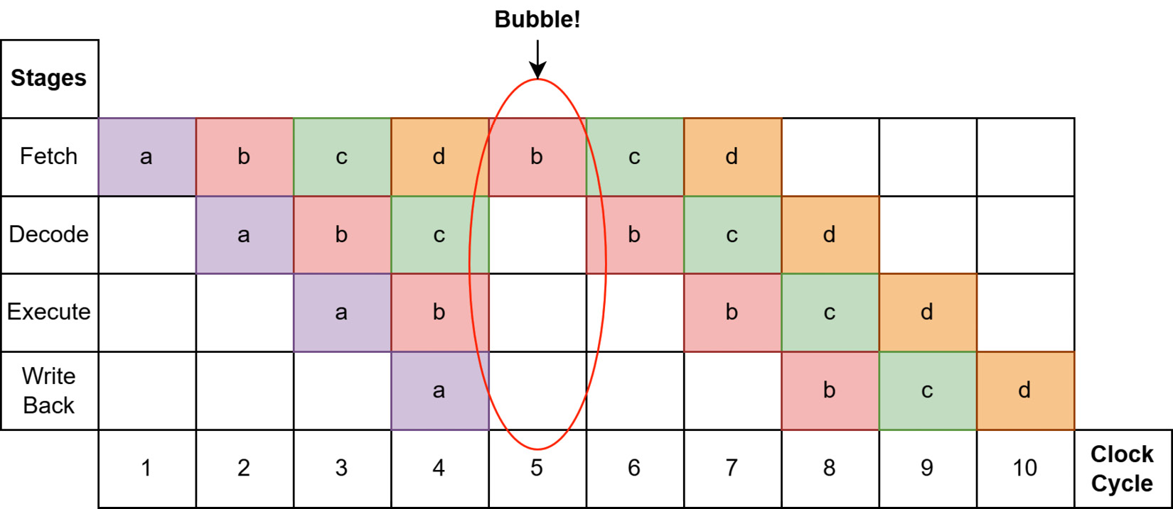
Figure 4.4 – CPU bubble misprediction

If executing instruction a results in a different branch of execution than what the processor predicted, the pipeline gets emptied and has to start over with the correct subsequent instruction. We can see in Figure 4.4 that the result is executing the same 4 instructions, but with a misprediction, takes 10 clock cycles instead of 7. Of course, this is an oversimplified example, but over time, lots of mispredictions can result in enormous differences in runtime by preventing the processor from maximizing its throughput. Taking advantage of this sort of processor-pipelining optimization is a significant principle of the Arrow libraries.

The hardware being used can affect your execution in other ways too. Traditional spinning-disk hard drives are notoriously slow for random reads compared to sequential reads, since this requires moving to another sector of the disk instead of just continuing to read from one sector. SSDs instead have very little-to-no overhead for random reads as opposed to sequential ones. When we talk about in-memory representations, the way that the operating system loads data into the main memory is the driving bottleneck for random reads versus sequential ones, as discussed in Chapter 1, Getting Started with Apache Arrow.

The more an in-memory representation keeps data in contiguous chunks of memory, the faster it is to load that data into registers for the CPU. A single instruction to load a large contiguous area of memory will be significantly faster than multiple instructions to load many different areas of memory. This led to the decision to use a column-oriented representation for Arrow, making it easier for the operating system and processor to make predictions about which memory will be needed for execution. The trade-off for this is that for some OLTP workloads, record-oriented structure representations such as FlatBuffers might be more performant than column-oriented ones. The important thing to remember is the difference in trade-offs and use cases between on-disk formats and ephemeral runtime in-memory representations. This is where we get to our last type of data format—those that are optimized for structured message passing.

Message-passing formats

The last class of formats we're going to talk about are message-passing formats such as Protobuf, FlatBuffers, and JSON again. In computer science, programming interfaces designed to allow coordination and message passing between different processes are referred to as inter-process communication (IPC) interfaces. For message passing and IPC, you want to optimize for small sizes since you're frequently passing the data across a network. In addition, being able to easily stream the data without losing contextual information is also a large benefit for these. In the case of Protobuf and FlatBuffers, you specify the schema in some external file and use a code generator to generate optimized message handling code. These technologies typically optimize for small message sizes and can start to become unwieldy or less performant when working with larger message sizes. For example, the official documentation for Protobuf says that it's optimal for message sizes to be less than 1 MB.

Despite the fact that the purpose of these formats is to pass messages rather than to be an optimized format for computation, the cost of serialization and deserialization as overhead is still extremely important. The faster that the data can be serialized and deserialized, the faster it can be sent and made available in the main memory for computations. This is one of the core reasons for Arrow's IPC format being raw data buffers with no serialization overhead, but the small metadata structures are passed using FlatBuffers in order to benefit from its high performance as a message-passing format.

If we compare Arrow to Protobuf or FlatBuffers, we can see that they are designed to solve two different problems. Protobuf and FlatBuffers provide a common representation for sending messages over the wire. Using the utilities provided and a schema, code for your preferred language can be generated to accept this common and compressed over-the-wire representation and convert it to an in-memory representation that can then be used. For passing smaller messages, this overhead of serialization and deserialization is relatively negligible. For use cases that need even better performance, FlatBuffers allows operations to be performed on the data without needing to copy from deserialized structures.

However, it's when we're looking at very large datasets that serialization and deserialization costs add up significantly and become a bottleneck. Moreover, you can't take the raw memory bytes that make up a Protobuf structure in C++ and then give those bytes to a Java program to use as-is. The structure needs to get serialized first by C++ to that common representation and then deserialized by Java into the in-memory representation that Java understands. This is why the Arrow format specification was created to have the same internal in-memory structure regardless of the language it is implemented in.

Summing up

If it wasn't already abundantly clear, to simplify the point: Arrow is not a competing technology with formats such as Protobuf for message passing, nor is it competing as an on-disk format with formats such as ORC or Parquet (despite it having a file format). The use case that Arrow targets is, instead, complementary. On-disk formats are designed for persistent, long-term storage on disk and require non-trivial amounts of work to decode and decompress the data before you can operate on it. Message-passing formats such as Protobuf are compacted by using tricks such as packing integer values together and tags to leave out optional fields with default values. This is to cut down on message sizes for fast transmission across networks; using Arrow as a small message-passing format would likely be less efficient.

Arrow is designed as an ephemeral, runtime in-memory format for processing data on a per-array-cell basis with minimal overhead. It is not intended for long-term, persistent storage, even though it has a file format for convenience. But when you do need to pass around Arrow record batches and tables of data, you're going to want to understand the Arrow IPC format and how to utilize it.

Passing your Arrows around

Since Arrow is designed to be easily passable between processes, regardless of whether they are locally on the same machine or not, the interfaces for passing around record batches are referred to as IPC libraries for Arrow. If the processes happen to be on the same machine, then it's possible to share your data without performing any copies at all!

What is this sorcery?!

First things first. There are two types of binary formats defined for sharing record batches between processes—a streaming format and a random access format, as outlined in more detail here:

• The streaming format exists for sending a sequence of record batches of an arbitrary length. It must be processed from start to end; you can't get random access to a particular record batch in the stream without processing all of the ones before it.
• The random access—or file—format is for sharing a known number of record batches. Because it supports random access to particular record batches, it is very useful in conjunction with memory mapping.

  Remember

  It's crucial to remember what a record batch is if you want to understand the format for sending binary Arrow data. A record batch is simply an ordered collection of arrays that all have the same length but potentially different data types. The field names, types, and metadata are collectively referred to as a record batch's schema.

Arrow's IPC protocol defines three message types used for conveying information: Schema, RecordBatch, and DictionaryBatch. The series of binary payloads for these messages can be reconstructed into in-memory record batches without the need for memory copying. Each message consists of a FlatBuffers message for metadata and an optional message body. FlatBuffers is a highly efficient, cross-platform serialization library designed originally by Google. The design of FlatBuffers provides for the message to be interpreted and accessed as-is without the need to deserialize it into a different intermediate format first. (You can learn more about FlatBuffers at https://google.github.io/flatbuffers/.)

The following diagram shows the format of encapsulated messages sent along the stream. The first 8 bytes consist of 0xFFFFFFFF to indicate a valid message followed by a 4-byte, little-endian (LE) integer value that indicates the size of the FlatBuffers message and the padding combined. Finally, the message is completed by the raw bytes of an optional message body whose length is a multiple of 8 bytes.

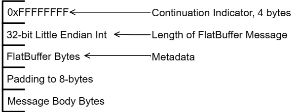
Figure 4.5 – IPC encapsulated message format

Okay; so, I know you're possibly thinking: Hey, didn't I read that there was no deserialization cost? Don't I have to unpack the FlatBuffer data? Well, the reason why FlatBuffers was chosen was that the binary data for fields in a FlatBuffer message can be accessed directly without having to unpack it into some other form. You only need the memory of the message itself to access the data; no additional allocations are necessary. Not only that, but it also even only requires part of the buffer to be in memory at a time if desired. Bottom line? It's fast! Also, keep in mind that you only have to deal with the FlatBuffer parts if you're actually implementing the specification; otherwise, all of this is just handled for you by the Arrow libraries.

So, let's take a look at the schema of a FlatBuffer message table, as follows:

table Message {

    version: org.apache.arrow.flatbuf.MetadataVersion;

    header: MessageHeader;

    bodyLength: long;

    custom_metadata: [ KeyValue ];

}

As you can see, the FlatBuffer message data contains a format version number, a specific message value (either Schema, RecordBatch, or DictionaryBatch), the length of the body in bytes, and a field for application-defined, key-value pairs of metadata. Generally, reading a stream of messages consists of reading the FlatBuffer message value first in order to obtain the size of the body, and then reading the body bytes. A typical stream will consist of a Schema message first, followed by some number of DictionaryBatch and RecordBatch messages. This doesn't contain any data buffers, only metadata information about the message, such as type information. We can visualize the stream of data like this:

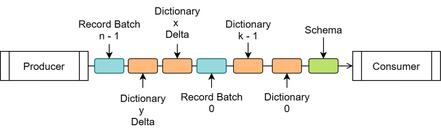
Figure 4.6 – Visualized IPC stream

Each box in the stream is an encapsulated message, as described before, containing the FlatBuffer data and optional body buffers. Dictionary messages would only show up in the stream if there are dictionary-encoded arrays in the schema. Each dictionary message contains an id field that is referenced by the schema to indicate which arrays use that dictionary, allowing optimization of using the same dictionary for multiple fields if possible, by referencing the id field for multiple arrays. In addition, there is an isDelta flag, allowing an existing dictionary to be expanded for subsequent record batches rather than having to resend the entire dictionary. Schema messages will contain no body data; they'll only contain the FlatBuffer message describing the types and metadata.

Record-batch messages contain the following:

• A header defined by the RecordBatch FlatBuffer message, containing the length and null count of each field in the record batch, along with the memory offset and length of each corresponding data buffer in the message body. To handle nested types, the fields are flattened into a pre-ordered depth-first traversal.
  • As an example, consider the following schema:
    • Col1: Struct<a: int32, b: List<item: float32>, c: float64>
    • Col2: String

The flattened version would look like this:

      Field0: Struct name='Col1'

      Field1: Int32 name='a'

      Field2: List name='b'

      Field3: Float32 name='item'

      Field4: Float64 name='c'

      Field5: UTF8 name='Col2'

• Raw buffers of data that make up the record batch, end to end and padded to ensure an 8-byte alignment:
  • For each flattened field in the record batch, the data buffers that make up the array would be based on the descriptions back in Chapter 1, Getting Started with Apache Arrow, which described which buffers exist based on the type: the validity bitmap, raw data, offsets, and so on.
  • When reading the message in, there's no need to copy or transform the data buffers; they can just be referred to as-is where they are without any copies or deserialization.

After each message in the stream, the reader can read the next 8 bytes to determine whether there is more data and the size of the following FlatBuffer metadata message. There are two possible ways for a writer to signal that there's no more data, or end of stream (EOS), as outlined here:

• Just closing the stream
• Writing 8 bytes that contain a 4-byte continuation indicator (0xFFFFFFFF) and then a length of 0 as a 4-byte integer for the next message (0x00000000)

There's just one more thing before we get to examples of actually using the IPC streams: the random-access file format. Trust me—if you understand the streaming format, the file format is really easy. The following diagram describes the file format:

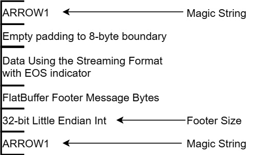
Figure 4.7 – IPC file format

The file format is really just an extension of the streaming format, with a magic string indicator to start and end the file, and a footer. The footer contains a copy of the schema (remember—the first message in the streaming format is also the schema) and the memory offsets and lengths for each block of data in the file, enabling random access to any record batch in the file. It is recommended to use the .arrow extension. A stream typically won't be written to a file, but if it is, the recommended extension is .arrow. There are also registered Multipurpose Internet Mail Extension (MIME) media types for both the streaming and file format of Apache Arrow data, as follows:

• https://www.iana.org/assignments/media-types/application/vnd.apache.arrow.stream
• https://www.iana.org/assignments/media-types/application/vnd.apache.arrow.file

  Extra Information

  There's an option in the IPC format that indicates that individual body buffers can be compressed in order to further reduce the size of the messages across the wire at the expense of some increased CPU usage. This could be very useful in cases where network latency is the bottleneck rather than CPU, or to reduce the file size if writing to a file. The two compression types supported by the IPC format are Zstandard (ZSTD) and Lempel-Ziv 4 (LZ4) compression.

Okay; we've covered the protocol for communicating Arrow data, so let's see some examples.

Producing and consuming Arrows

What if you wanted to build a service that read in remote files and streamed the data back to the client? Seems simplistic, but it is the basis of a lot of data transfer use cases if you toss a variety of data manipulation in between the reading of the data files and streaming the data along. So, we're going to build something similar to this:

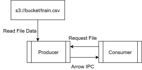
Figure 4.8 – Simple server-consumer IPC example

By following Figure 4.8, we see the following steps:

1. The consumer requests a file (not covered here, but will exist in GitHub samples).
2. Establishing an input stream from S3 to read the file as Arrow record batches.
3. Writing record batches to the consumer as we read them in from S3.

Should we take a stab at this, then? Here we go!

We've already covered reading files from S3 in Python and C++, so let's write the example for the producer side using Go, as follows:

1. First, we need our imports, as shown here:

   import (

       "context"

           …

       "github.com/apache/arrow/go/v7/arrow"

       "github.com/apache/arrow/go/v7/arrow/csv"

       "github.com/apache/arrow/go/v7/arrow/ipc"        

       "github.com/aws/aws-sdk-go-v2/aws"

       "github.com/aws/aws-sdk-go-v2/service/s3"

   )

2. Next, we can create our S3 client and establish our input stream, as follows:

   client := s3.New(s3.Options{Region: "us-east-1"})

   obj, err := client.GetObject(context.Background(),

         &s3.GetObjectInput{

              Bucket: aws.String("nyc-tlc"),

              Key: aws.String("trip data/yellow_tripdata_2020-11.csv")})

   if err != nil {

      // handle the error

   }

Assuming there were no errors, there is a member called Body on the obj return that will be a stream to read the data for the file.

3. Now, we can set up our CSV reader, as follows:

   schema := arrow.NewSchema([]arrow.Field{

       // put the expected schema of the CSV file

   }, nil)

   headerline := true // set to false if first line is not

                      // the column headers

   reader := csv.NewReader(obj.Body, schema,

       csv.WithHeader(headerline))

   defer reader.Release()

You can see the documentation to find other possible options that exist for creating a CSV reader.

4. To set up our IPC stream, we create an ipc.Writer interface and pass it a stream to write to. It could be anything that meets the io.Writer interface, whether it's a file or a HyperText Transfer Protocol (HTTP) response writer. The code is illustrated in the following snippet:

   // assume w is our stream to write to

   writer := ipc.NewWriter(w, ipc.WithSchema(reader.Schema()))

   defer writer.Close()

5. Finally, we can just read in record batches and write them out as we go! This is what the process looks like:

   for reader.Next() {

       if err := writer.Write(reader.Record()); err != nil {

           // handle the error

           break

       }

   }

   if reader.Err() != nil {

       // we didn't stop because we're done, we stopped because

       // the reader had an error, handle the error!

   }

And that's that!

Consuming this stream is also easy to do regardless of the programming language you're using. Conceptually, all the following work in the same way as they pertain to reading and writing the IPC format:

• With Go, you'd use ipc.Reader.
• For Python, there is pyarrow.RecordBatchStreamReader, and writing would be done with pyarrow.RecordBatchStreamWriter.

The reader also has a special read_pandas function to simplify the case where you might want to read many record batches and convert them to a single DataFrame.

• The C++ library provides arrow::ipc::RecordBatchStreamReader::Open, which accepts arrow::io::InputStream to create a reader, and arrow::ipc::MakeStreamWriter for creating a writer from arrow::io::OutputStream.

If you'd prefer to use the random-access file format, then each of the preceding functions has corresponding versions for reading and writing the file format instead. If you're storing DataFrames or Arrow tables as files, you may have come across functions or documentation mentioning the Feather file format. The Feather file format is just the Arrow IPC file format on disk and was created early on during the beginnings of the Arrow project as a proof of concept (PoC) for language-agnostic DataFrame storage for Python and R. Originally, the formats were not identical (the version 1 (V1) Feather format), so there still exist functions in the pyarrow and pandas libraries for specifically reading and writing Feather files (that will default to the V2 format, which is exactly the current Arrow IPC format).

To ensure efficient memory usage when dealing with all these streams and files, the Arrow libraries all provide various utilities for memory management that are also utilized internally by them. These helper classes and utilities are what we're going to cover next so that you'll know how to take advantage of them to make your scripts and programs as lean as possible. We're also going to cover how you can share your buffers across programming language boundaries for improved performance, and why you'd want to do so.

The Arrow IPC file format, or Feather, was created to provide performance benefits through memory mapping. Because the Arrow IPC format has raw data buffers precisely in the same way they would be in memory, a technique called memory mapping can be utilized to minimize memory overhead for processing. Let's see what that is and how it works!

Learning about memory cartography

One draw of distributed systems such as Apache Spark is the ability to process very large datasets quickly. Sometimes, the dataset is so large that it can't even fit entirely in memory on a single machine! Having a distributed system that can break up the data into chunks and process them in parallel is then necessary since no individual machine would be able to load the whole dataset in memory at one time to operate on it. But what if you could process a huge, multiple-GB file while using almost no RAM at all? That's where memory mapping comes in.

Let's look to our NYC Taxi dataset once again for help with demonstrating this concept. The file named yellow_tripdata_2015-01.csv is approximately 1.8 GB in size, perfect to use as an example. By now, you should easily be able to read that CSV file in as an Arrow table and look at the schema. Now, let's say we wanted to find out and calculate the mean of the values in the total_amount column. For the ease and brevity of code snippets, we'll use the Python Arrow library for this example.

Acquiring the Data

You can download the sample file we're using here from the public-facing Amazon Web Services (AWS) S3 bucket at this URL: https://s3.amazonaws.com/nyc-tlc/trip+data/yellow_tripdata_2015-01.csv.

The base case

In order to see how much benefit we get out of memory mapping, we first need to construct our base case. We need to first calculate the mean of the values in the total_amount column without memory mapping so that we have a baseline for the runtime and memory usage. Using the pyarrow library and pandas, if you remember from Chapter 3, Data Science with Apache Arrow, there are two easy ways to calculate the total_amount column of the CSV file. One is significantly slower than the other. Do you remember what they are? Have a look at the following code snippet:

In [0]: import pandas as pd

In [1]: %%timeit

   ...: pd.read_csv('yellow_tripdata_2015-01.csv')['total_amount'].mean()

   ...:

As usual, because we used the special %%timeit function, we get the time that it took to execute output below the results in IPython. On my laptop, the timing output from IPython shows it taking 20.2 seconds, give or take 400 milliseconds, to do this. This is the slow way. See if you remember the fast way; I'll still be here when you get back.

Figured it out? I hope so! But for those who didn't, here it is:

In [2]: import pyarrow as pa

In [3]: import pyarrow.csv

In [4]: %%timeit

   ...: df = pa.csv.read_csv('yellow_tripdata_2015-01.csv',

   ...:      convert_options=pa.csv.ConvertOptions(

   ...:    include_columns=['total_amount'])).to_pandas()

   ...: df.mean()

   ...:

When I run this, it takes 816 milliseconds—plus or minus 27 milliseconds—on my laptop. We now have our base-case time that it takes to get the mean value of the total_amount column from our 1.8 GB CSV file. The next step for our comparison is to write the data out to a Parquet file instead of a CSV file and see how it compares for us to read the single column and calculate the mean.

Parquet versus CSV

When written as a Parquet file using the default settings, the table of data from the yellow_tripdata_2015-01.csv file clocks in at just over 282 MB. Just as I said earlier, binary formats allow for higher compression ratios among the other compression techniques that Parquet utilizes. We can then use the Parquet file to see how the smaller file size and I/O benefits of Parquet can let us improve the performance of the computation. Let's try calculating the same mean of the column, but this time using the Parquet file instead of the CSV file, as follows:

In [5]: %%timeit

   ...: pd.read_parquet('yellow_tripdata_2015-01.parquet', 

   ...: columns=['total_amount']).mean()

   ...:

As I mentioned before, we can take advantage of the fact that Parquet allows us to only read the column we want rather than having to read everything, as we do with CSV. Combining the smaller size of the compressed data and the reduction in I/O by only having to read a single column of data, my laptop reports that this takes about 230 milliseconds. That's around 3.5 times faster than calculating it from the CSV file using pyarrow, and 87 times faster than using pandas directly. Depending on whether you're using an SSD, Non-Volatile Memory Express (NVMe), or spinning-disk hard drive, your performance may vary.

Before we move on, let's look at the data we have compiled so far. Here it is:

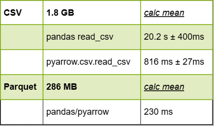
Figure 4.9 – File size and performance numbers (CSV and Parquet)

Now let's try using a memory-mapped file.

Mapping data into memory

I'll go into the mechanics of what exactly is happening behind the scenes a little later in the chapter, but for now, we'll examine how to use memory mapping with the Arrow libraries. In order to benefit from the memory map, we need to write the file out as an Arrow IPC file. Let's use RecordBatchFileWriter to write out our table, as follows:

In [6]: table = pa.csv.read_csv('yellow_tripdata_2015-01.csv').combine_chunks() # we want one contiguous table

In [7]: with pa.OSFile('yellow_tripdata_2015-01.arrow', 'wb') as sink:

   ...:     with pa.RecordBatchFileWriter(sink, table.schema) as writer:

   ...:         writer.write_table(table)

   ...:

Notice the use of the .arrow extension to denote the file. This follows the standard media types that are recognized by the Internet Assigned Numbers Authority (IANA). By default, this file is not compressed in any way, which means that it's pretty big. While the CSV file is around 1.82 GB, the Arrow IPC file ends up being around 1.77 GB, roughly only around 50 MB difference. We can then map the file into memory and do the same thing we did earlier to calculate the mean from the Arrow table, as follows:

In [8]: %%timeit

   ...: source = pa.memory_map('yellow_tripdata_2015-01.arrow')

   ...: table = pa.ipc.RecordBatchFileReader(source).read_all().column('total_amount')

   ...: result = table.to_pandas().mean()

   ...:

This clocks in at a very speedy 200 milliseconds on my laptop, which is quite nice. The following screenshot shows an updated version of the table from Figure 4.9, now including our Arrow IPC file:

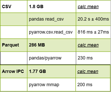
Figure 4.10 – File size and performance, including memory mapping

To really see the benefit, we need to check how much memory is being allocated and used by the process for each of these approaches. In order to do this, we'll need to install the psutil package using pip, as follows:

$ pip install psutil

To check the memory usage of the approaches, we can just check the currently allocated memory by the process before and after each read and check the difference. We can put a script together that does this rather than using IPython or Jupyter and doing it interactively. Let's walk through the script, starting with the first line, as follows:

# initial memory usage in megabytes

memory_init = psutil.Process(os.getpid()).memory_info().rss >> 20

We check the current memory usage of the process using the psutil library and convert the value from bytes to MB for easy reading. Now, we can just read the data and get the column we wanted in various ways, storing the current memory usage after each one, first by reading the CSV file and taking just the column we want from the resulting table, as follows:

col_pd_csv = pd.read_csv('yellow_tripdata_2015-01.csv')['total_amount']

memory_pd_csv = psutil.Process(os.getpid()).memory_info().rss >> 20

Then, we pass the column in as an option to prune unnecessary columns earlier in the processing, as follows:

col_pa_csv = pa.csv.read_csv('yellow_tripdata_2015-01.csv',

                 convert_options=pa.csv.ConvertOptions(

             include_columns=['total_amount'])).to_pandas()

memory_pa_csv = psutil.Process(os.getpid()).memory_info().rss >> 20

Now, we use the Parquet file instead of the CSV file, as follows:

col_parquet = pd.read_parquet('yellow_tripdata_2015-01.parquet', columns=['total_amount'])

memory_parquet = psutil.Process(os.getpid()).memory_info().rss >> 20

Then, we use the Feather—or Arrow IPC—file, but without memory mapping, as follows:

with pa.OSFile('yellow_tripdata_2015-01.arrow', 'rb') as source:

     col_arrow_file = pa.ipc.open_file(source).read_all().column(

                              'total_amount').to_pandas()

memory_arrow = psutil.Process(os.getpid()).memory_info().rss >> 20

It's important to note that the whole .arrow file needs to be loaded in via read_all before you can filter on a single column. This is where memory-mapping the Arrow IPC file can come in handy! Memory mapping the file allows us to reference locations in the file that contain the column data we want without having to load it in. Getting the column by memory mapping the Arrow IPC file looks like this:

source = pa.memory_map('yellow_tripdata_2015-01.arrow', 'r')

table_mmap = pa.ipc.RecordBatchFileReader(source).read_all().column(

              'total_amount')

col_arrow_mmap = table_mmap.to_pandas(zero_copy_only=True)

memory_mmapped = psutil.Process(os.getpid()).memory_info().rss >> 20

The highlighted lines in the preceding code snippet each show the variables we store the memory usage in after each time we read the data. If we progressively subtract the values, we can see how much memory was allocated by the process for each way of getting the data. In order of appearance in the script, this is how we get the memory usage value for each of the ways we tried reading in the column:

1. With pandas, read CSV: memory_pd_csv – memory_init
2. Read CSV using pyarrow: memory_pa_csv – memory_pd_csv
3. Read Parquet column: memory_parquet – memory_pa_csv
4. Read Arrow file normally: memory_arrow – memory_parquet
5. Read memory-mapped Arrow IPC file: memory_mmapped – memory_arrow

And now, the moment of truth! How much memory did each approach use? Let's take a look:

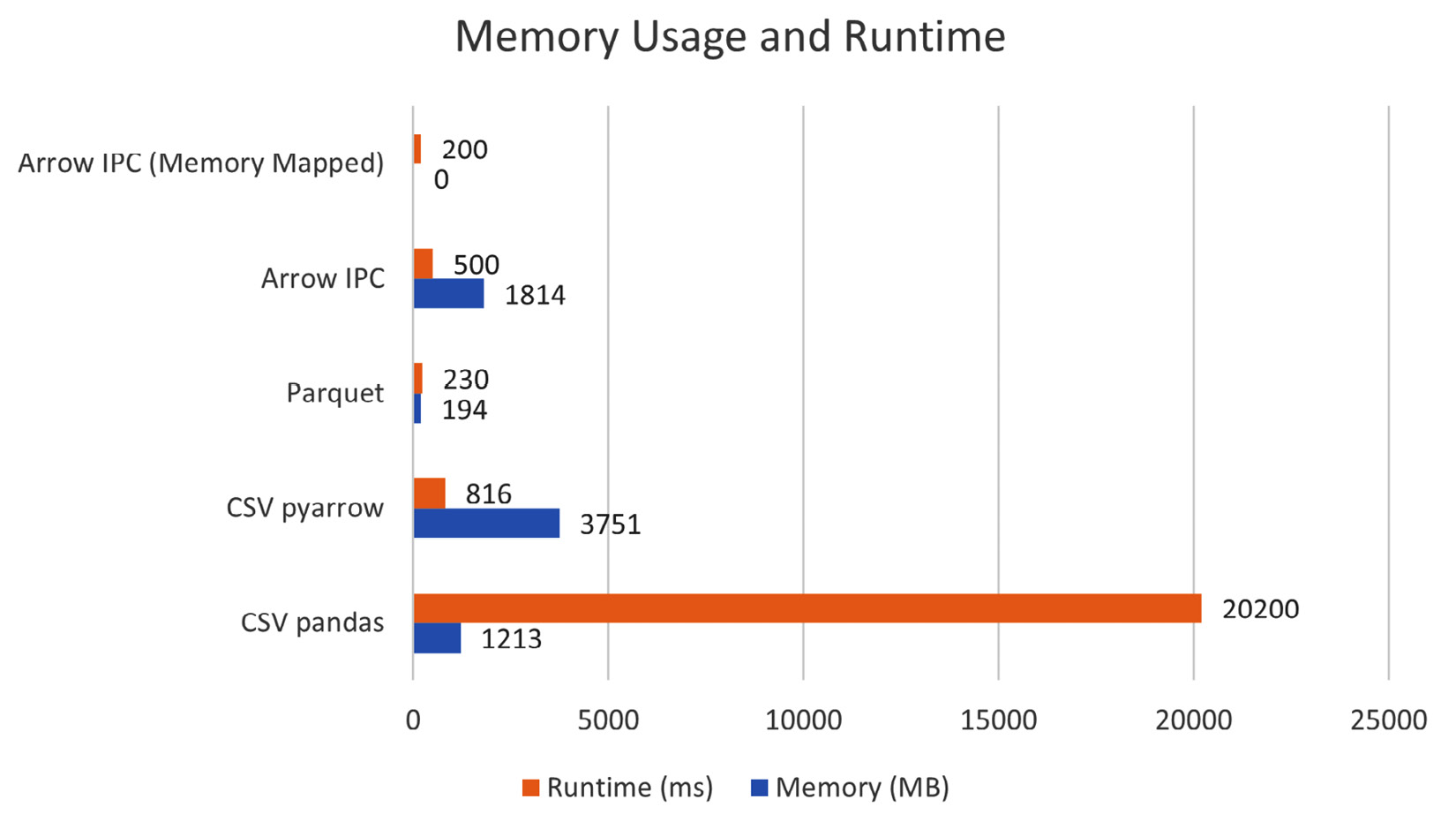
Figure 4.11 – Memory usage and runtime to calculate the mean

There we have it—by using a memory-mapped file, even though it's a 1,814 MB file, there's effectively zero physical memory allocated to read in the column. Magic! We can also see that the memory usage for reading the Arrow IPC file normally is the entire file size because it has to read the whole file into memory to process it. Meanwhile, Parquet uses a very respectable 194 MB only. The real shocking one is reading in the file using the pyarrow library, just over twice the size of the file used as memory. This is because the multithreaded reads don't allocate a single contiguous chunk of memory but instead multiple smaller chunks. So, when we create the pandas DataFrame, it needs to insert a copy of the data into a contiguous memory location. We're sacrificing memory for performance as compared to the single-threaded version of reading the file, but then have to pay the cost of allocating all that memory.

There are two reasons why the memory-mapped file approach ends up being faster than the Parquet version: not having to allocate any memory, and no decoding is necessary to access the data. We just reference the memory as-is and can work with it immediately!

If you're curious about how this magical sorcery works, then read on, my adventurous reader!

Too long; didn't read (TL;DR) – Computers are magic

Before I can explain the sorcery behind memory mapping, you have to understand how memory for a running process works. There's going to be a bit of oversimplification here, and that's okay! This is a crash course, not a college class.

Virtual and physical memory space

Most modern operating systems use the concept of virtualized memory for handling the memory used for a running process. This means that the entirety of the space of addresses that a process might reference doesn't have to be stored in the physical RAM on the device all the time. Instead, the operating system can swap data from the process' memory out of the main memory, and write pages to a pagefile or a cache, or any other way it wants to handle it. In this context, think of a page of data as just a chunk of memory, frequently around 4 kilobytes (KB). The operating system then maintains a mapping table, known as a page table, which maps the virtual addresses to physical locations in RAM where that data is stored. If a request is made to load data that isn't physically in RAM, it's called a page fault. The requested data is then swapped back into RAM so that it can be referenced properly by the process. This is all invisible to the process and is handled at the operating-system level. You can see an illustration of the process in the following diagram:

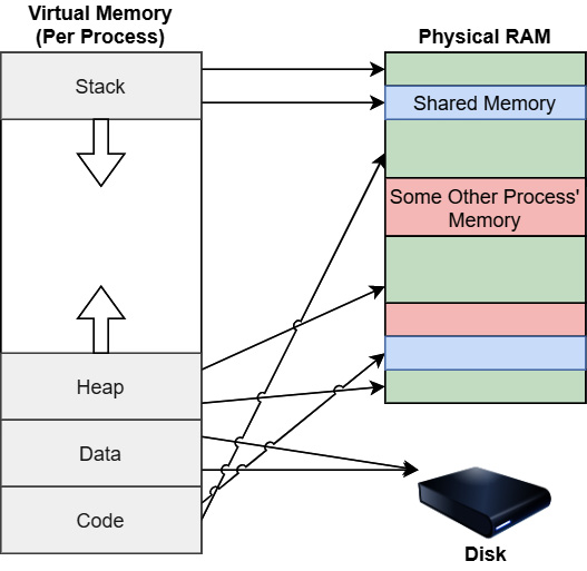
Figure 4.12 – Virtual and physical memory

Figure 4.12 shows a diagram of how a process' view of its virtual memory might map to physical memory and the disk. The process gets to see its memory as if it's a contiguous space that has its stack, heap, shared libraries, and anything else it has to reference in memory. But physically, chunks of that memory can exist in various locations on the RAM chips or even on disk in a pagefile or a cache somewhere. The operating system then keeps track of the mappings between the virtual-memory locations and the physical locations of the memory, updating that table as it moves data into and out of the physical RAM on-demand by processes.

There are various benefits to virtualized memory that have made it the de facto standard, some of which are listed here:

• Processes don't need to manage shared memory spaces themselves.
• The operating system can leverage shared libraries between processes to share the same memory spaces and reduce overall memory consumption.
• Increased security by isolating one process' memory from another process.
• Being able to conceptually reference and manipulate more memory than is physically available.

When you read data from a file, your process makes a system call that then has to pass through various drivers and memory managers every time you want to read or write data to the file. At many steps along the way, that data gets buffered and cached (read copied). Memory mapping a file allows us to bypass all those copies and treat the data of a file as if it were normal memory with load/store calls as opposed to system calls, which are orders of magnitude slower.

What does memory mapping do?

Memory mapping is functionality that is provided by the Portable Operating System Interface (POSIX)-defined mmap function on many operating systems. When you memory map a file, a chunk of the virtual address space for the process equivalent to the size of the file is blocked out, allowing the process to treat the file data as simple memory loading and storing. In most cases, the region of memory that is mapped is directly the kernel's page (file) cache, which means that no copies get created when accessing the data.

The following diagram shows an example of a situation when a file is memory-mapped. All accesses to a file go through the kernel's page cache so that updates to the mapped file are immediately visible to any processes that attempt to read the file, even though they won't exist physically on the device until the buffers are flushed and synced back to the physical drive. This means that multiple processes can memory map the same file and treat it as a region of shared memory, which is how dedicated shared process memory is often implemented under the hood.

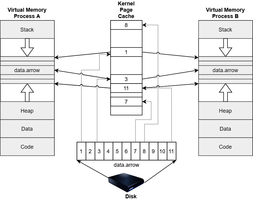
Figure 4.13 – Memory-mapped file-page cache

In our example of memory mapping, the large Arrow file to read the values and process the column, we're taking advantage of the lazy loading and zero-copy properties of memory mapping and the pyarrow library. By memory mapping the 1.77 GB file, the library is able to treat the file as if it were already in memory without having to actually allocate the entire 1.77 GB of the file. It will only read the pages from the file that it needs when the corresponding virtual memory locations are accessed. In the meantime, we can just pass references to the memory addresses around. We read a few KB of data from the bottom of the file, which, as you'll remember from Chapter 1, Getting Started with Apache Arrow, is where the metadata and schema will be stored, accessing only the corresponding pages. When we finally want to read the values in the column in order to perform a computation, only then will the data be materialized and pulled into RAM. The code snippet from the Mapping data into memory section, when we measured the memory usage, didn't perform the mean calculations; it only read the data into pandas DataFrame objects. Since we never tried to read the data in the column, the only data pulled into memory from the file was the few KB of metadata.

If we add the highlighted line to perform the mean calculation, then we'll see the memory usage for reading from the file, as follows:

source = pa.memory_map('yellow_tripdata_2015-01.arrow', 'r')

table_mmap = pa.ipc.RecordBatchFileReader(source).read_all().column(

              'total_amount')

col_arrow_mmap = table_mmap.to_pandas(zero_copy_only=True)

result = col_arrow_mmap.mean()

memory_mmapped = psutil.Process(os.getpid()).memory_info().rss >> 20

Running the script with this added line results in an output saying that it now uses 97 MB instead of 0, which is exactly what you get when you multiply the number of rows (12,748,986) by the size of a double (8 bytes). To calculate the mean of the column from the 1.77 GB file, we were able to only require as much RAM as the column itself to perform the aggregation calculation—just 97 MB. Pretty cool, right?

So, why don't we just always memory map files? Well, it's not as simple as that. Let's find out why.

Memory mapping is not a silver bullet

As we saw in the preceding sections, the primary reason to use a persistent memory-mapped file is for I/O performance. But as with everything, it's still a trade-off. While the standard approach for I/O is slow due to the overhead of system calls and the copying of memory, memory-mapped I/O also has a cost: minor page faults. A page fault happens when a process attempts to access a page of its virtual memory space that hasn't yet been loaded into memory. In the case of memory-mapped I/O, a minor page fault is when a page exists in memory, but the memory management unit of the system hasn't yet marked it as being loaded when it is accessed by the process. This would happen when a block of data has been loaded into the page cache, such as in Figure 4.13, but has not yet been mapped and connected to the appropriate location in the process' virtual memory space. Depending on the access pattern and hardware, in some circumstances, memory-mapped I/O can be significantly slower than standard I/O.

For very small files, in the order of KB or smaller, memory mapping them can end up causing excess memory fragmentation and result in a waste of memory space. Memory-mapped regions are always going to be aligned to the memory page size, which is frequently around 4 KB in most systems. Once the whole file is loaded into memory, mapping a 5 KB file will require 2 memory pages, or 8 KB of allocated memory. The following diagram shows how this then results in 3 KB of wasted slack space in memory:

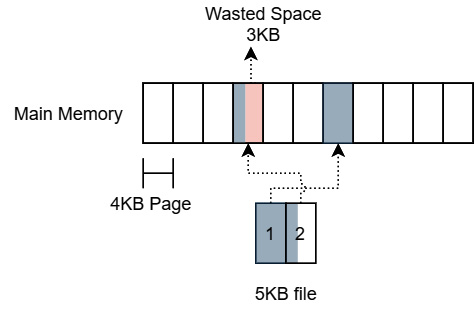
Figure 4.14 – Wasted space memory mapping small files

While 3 KB might not seem like a lot of memory space, if you memory map a large number of small files, this can add up to a lot of fragmentation and wasted memory space. Finally, when you have extremely fast devices, such as modern NVMe SSDs, you can wind up getting limited by the fact that many operating systems limit the number of CPU cores that handle page faults. The result is that memory-mapped I/O ends up being less scalable than standard I/O. With too many processes performing memory mapping, you can end up bottlenecked by this cap on cores rather than by the storage device.

There are a few other considerations that need to be kept in mind when using memory-mapped files, as outlined here:

• Any I/O error on the backing source file while accessing the mapped memory gets reported to the process as errors that wouldn't normally occur when just accessing memory. When working with memory-mapped I/O, all code accessing the mapped memory should be prepared to handle those errors.
• On hardware without a memory management unit, such as embedded or lower-power systems, the operating system can copy the entire file into memory when a request is made to map it. This obviously can only work for files that will fit in the available memory and would be slow if you only need to access a small portion of the file.

All in all, memory mapping is a crucial technique for handling very large files that you only need to read small portions of and for sharing memory between processes. Just make sure you test and benchmark frequently to ensure you're actually getting a benefit from it. Keep in mind that memory mapping things such as Parquet files is less beneficial than mapping raw Arrow IPC files. You may ask: Why is that? Since the data in the Parquet file still needs to be decoded and decompressed before you can use it, memory still needs to get allocated to hold the decoded data. While you might save a small amount of performance on the I/O costs of the Parquet file, on a sufficiently fast disk, the bottleneck will be the memory allocations and CPU for decoding and decompressing instead. The raw bytes of Arrow IPC files, on the contrary, can be used in memory directly as they are, as we saw earlier, bypassing the need for any additional memory allocations to use and reference the data from the file.

Summary

If you are building up data pipelines and large systems, regardless of whether you are a data scientist or a software architect, you're going to have to make a lot of decisions regarding which formats to use for various pieces of the system. You always want to choose the best format for the use case, and not just pick the latest trends and apply them everywhere. Many people hear about Arrow and either react by thinking that they need to use it everywhere for everything, or they wonder why we needed yet another data format. The key takeaway I want you to understand is the differences in the problems that are trying to be solved.

If you need longer-term persistent storage either on disk or in the cloud, you typically want a storage format such as Parquet, ORC, or CSV, with the primary access cost being I/O time for these use cases, so you want to optimize to reduce that based on your access patterns. If you're passing small messages around, such as metadata or control messages, then formats such as Protobuf, FlatBuffers, and JSON will potentially be optimal. You don't want to use this for large tabular datasets, though, especially if you will need to perform analytics and computations on the data. These are not hard-and-fast rules—they are guidelines. The use case that Arrow targets is to be an in-memory ephemeral runtime format for data, providing a shared-memory format so that more CPU time can be spent on performing computations rather than on having to convert large amounts of data between different formats as it passes through a system.

Hopefully, you've also picked up ideas for optimizing your memory usage when it comes to dealing with these large files and data handling, such as when it might make sense to use Arrow IPC files instead of compact Parquet files or otherwise. As I said, make sure to use the right format to solve the problem in front of you given all of the factors: the hardware, the networks, the data, and the process itself.

The next chapter is titled Crossing the Language Barrier with the Arrow C Data API. Up till now, we've covered a lot of the surface information, creating arrays and tables, reading and writing files in various formats, and so on. But remember: I said that Arrow is a collection of libraries for handling data. We're going to dive deeper and look at some of the more experimental APIs that the Arrow libraries expose, such as the Compute API. This chapter was kind of light on code; the next chapter will not be. I hope you stick around!

See you on the next page!