
Chapter 7: Using the Arrow Datasets API
In the current ecosystem of data lakes and lakehouses, many datasets are now huge collections of files in partitioned directory structures rather than a single file. To facilitate this workflow, the Arrow libraries provide an API for easily interacting with these types of structured and unstructured data. This is called the Datasets API and is designed to perform a lot of the heavy lifting for querying these types of datasets for you.
The Datasets API provides a series of utilities for easily interacting with large, distributed, and possibly partitioned datasets that are spread across multiple files. It also integrates very easily with the Compute APIs we covered previously, in Chapter 6, Leveraging the Arrow Compute APIs.
In this chapter, we will learn how to use the Arrow Datasets API for efficient querying of multifile, tabular datasets regardless of their location or format. We will also understand how to use the dataset classes and methods to easily filter or perform computations on arbitrarily large datasets.
Here are the topics that we will cover:
- Querying multifile datasets
- Filtering data programmatically
- Using the Datasets API in Python
- Streaming results
Technical requirements
As before, this chapter has a lot of code examples and exercises to drive home an understanding of using these libraries. You'll need an internet-connected computer with the following to try out the examples and follow along:
- Python 3+: With the pyarrow module installed and the dataset submodule.
- A C++ compiler supporting C++11 or higher: With the Arrow libraries installed and able to be included and linked against.
- Your preferred coding IDE, such as Emacs, Vim, Sublime, or VS Code.
- As before, you can find the full sample code in the accompanying GitHub repository at https://github.com/PacktPublishing/In-Memory-Analytics-with-Apache-Arrow-.
- We're also going to utilize the NYC taxi dataset located in the public AWS S3 bucket at s3://ursa-labs-taxi-data/.
Querying multifile datasets
Note
While this section details the Datasets API in the Arrow libraries, it's important to note that this API is still considered experimental as of the time of writing. As a result, the APIs described are not yet guaranteed to be stable between version upgrades of Arrow and may change in some ways. Always check the documentation for the version of Arrow you're using. That said, the API is unlikely to change drastically unless requested by users, so it's being included due to its extreme utility.
To facilitate the very quick querying of data, modern datasets are often partitioned into multiple files across multiple directories. Many engines and utilities take advantage of this or read and write data in this format, such as Apache Hive, Dremio Sonar, Presto, and many AWS services. The Arrow datasets library provides functionality as a library for working with these sorts of tabular datasets, such as the following:
- Providing a single, unified interface that supports different data formats and filesystems. As of version 7.0.0 of Arrow, this includes Parquet, ORC, Feather (or Arrow IPC), and CSV files that are either local or stored in the cloud, such as S3 or HDFS.
- Discovering sources by crawling partitioned directories and providing some simple normalizing of schemas between different partitions.
- Predicate pushdown for filtering rows efficiently along with optimized column projection and parallel reading.
Using the trusty NYC taxi dataset again, let's see an example of how you might partition this data for easier querying. The most obvious, and most likely, way that this data would get partitioned is by date, specifically, by year and then by month. Figure 7.1 shows what this might look like:
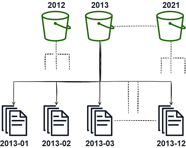
Figure 7.1 – Sample partition scheme, year/month
Partitioning the data in this way allows us to utilize the directories and files to minimize the number of files we actually have to read to satisfy a query that is requesting a particular time frame. For example, if a query is requesting information about the data for the entire year of 2015, we're able to skip reading any files that aren't in the 2015 bucket. The same would go for a query about data from year to year but only in January; we'd be able to simply read only the 01 file in each year's bucket.
In the case of the NYC taxi dataset, another potential way to partition the data would be to partition it by the source type first and then by year and month. Whether or not it makes sense to do this depends on the query pattern that you're expecting to serve. If the majority of the time you're only querying one type (yellow, green, fhv, and so on), then it would be highly beneficial to partition the dataset in this way, as shown in Figure 7.2. If instead the queries will often mix the data between the dataset types, it might be better to keep the data only partitioned by year and month to minimize the I/O communication:
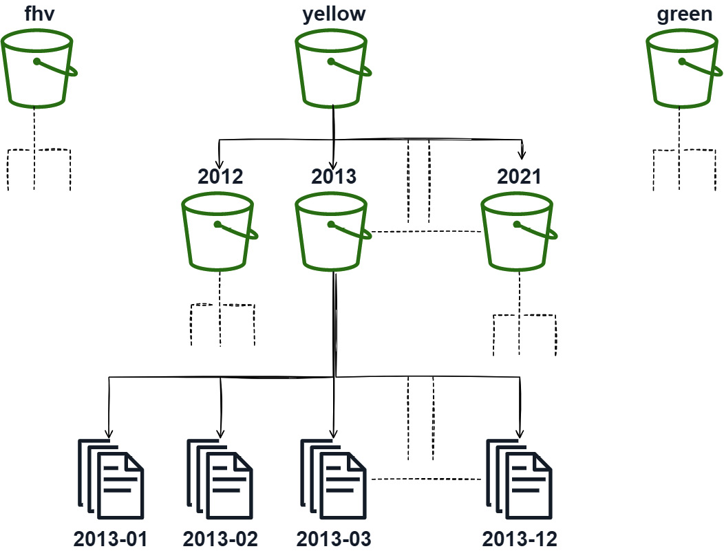
Figure 7.2 – Multikey partition
This partitioning technique can be applied for any columns that are frequently filtered on, not just the obvious ones, such as date and dataset type. It's making a trade-off between improving the filtering by reducing the number of files to read in and having potentially more files to read when not filtering on that column.
But we're getting ahead of ourselves here. Let's start with a simple example and work from there.
Creating a sample dataset
The first thing we're going to do is to create a sample dataset consisting of a directory containing two Parquet files. For simplicity, we can just have three int64 columns named a, b, and c. Our whole dataset can look like Figure 7.3, which shows the two Parquet files. Before looking at the code snippet, try coding up something to write the two files yourself in the language of your choice:
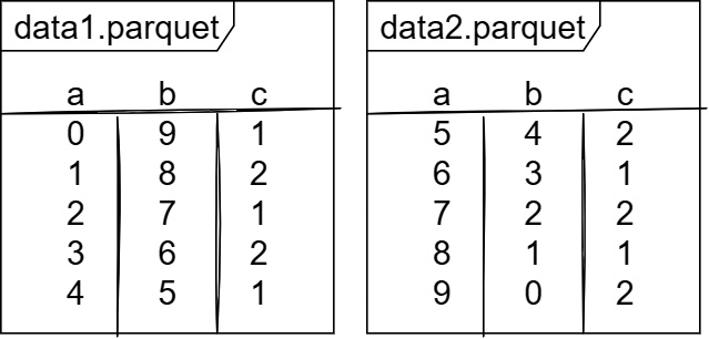
Figure 7.3 – Sample dataset
Here's a code snippet that will produce those two files just as we want them. I'll use C++ for this example but you can use whichever language you want. There are also Python versions of these in the accompanying GitHub repository for you to peruse:
- First, here's a small helper macro to abort on an error:
#include <arrow/api.h>
#include <iostream>
#define ABORT_ON_FAIL(expr)
do {
arrow::Status status_ = (expr);
if (!status_.ok()) {
std::cerr << status_.message()
<< std::endl;
abort();
}
} while(0);
- We'll make a create_table function next for simplicity:
#include <memory>
std::shared_ptr<arrow::Table> create_table() {
auto schema =
arrow::schema({arrow::field("a", arrow::int64()),
arrow::field("b", arrow::int64()),
arrow::field("c", arrow::int64())});
std::shared_ptr<arrow::Array> array_a, array_b, array_c;
arrow::NumericBuilder<arrow::Int64Type> builder;
builder.AppendValues({0, 1, 2, 3, 4, 5, 6, 7, 8, 9});
ABORT_ON_FAIL(builder.Finish(&array_a));
builder.Reset();
builder.AppendValues({9, 8, 7, 6, 5, 4, 3, 2, 1, 0});
ABORT_ON_FAIL(builder.Finish(&array_b));
builder.Reset();
builder.AppendValues({1, 2, 1, 2, 1, 2, 1, 2, 1, 2});
ABORT_ON_FAIL(builder.Finish(&array_c));
builder.Reset();
return arrow::Table::Make(schema,
{array_a, array_b, array_c});
}
- Then, add a function to write the Parquet files from the table we create:
#include <arrow/filesystem/api.h>
#include <parquet/arrow/writer.h>
namespace fs = arrow::fs;
std::string create_sample_dataset(
const std::shared_ptr<fs::FileSystem>& filesystem,
const std::string& root_path) {
auto base_path = root_path + "/parquet_dataset";
ABORT_ON_FAIL(filesystem->CreateDir(base_path));
auto table = create_table();
auto output =
filesystem->OpenOutputStream(base_path +
"/data1.parquet").ValueOrDie();
ABORT_ON_FAIL(parquet::arrow::WriteTable(
*table->Slice(0, 5),
arrow::default_memory_pool(),
output, /*chunk_size*/2048));
output = filesystem->OpenOutputStream(base_path +
"/data2.parquet").ValueOrDie();
ABORT_ON_FAIL(parquet::arrow::WriteTable(
*table->Slice(5),
arrow::default_memory_pool(),
output, /*chunk_size*/2048));
return base_path;
}
- Finally, we add a main function to initialize the filesystem and set a root path:
int main() {
std::shared_ptr<fs::FileSystem> filesystem =
std::make_shared<fs::LocalFileSystem>();
auto path = create_sample_dataset(filesystem,
"/home/matt/sample");
std::cout << path << std::endl;
}
Of course, replace the root path to write to with the relevant path for you.
Discovering dataset fragments
The Arrow Dataset library is capable of discovering the files that exist for a filesystem-based dataset for you, without requiring you to describe every single file path that is part of it. The current concrete dataset implementations as of version 7.0.0 of the Arrow library are as follows:
- FileSystemDataset: Dataset constructed of various files in a directory structure
- InMemoryDataset: Dataset consisting of a bunch of record batches that already exist in memory
- UnionDataset: Dataset that consists of one or more other datasets as children
When we talk about fragments of a dataset, we're referring to the units of parallelization that exist for the dataset. For InMemoryDataset, this would be the individual record batches. Most often, for a filesystem-based dataset, the "fragments" would be the individual files. But in the case of something such as Parquet files, a fragment could also be a single row group from a single file too. Let's use the factory functions that exist in the library to create a dataset of our two sample Parquet files:
- Let's get our include directive and function signature set up first:
#include <arrow/dataset/api.h>
namespace ds = arrow::dataset; // convenient
std::shared_ptr<arrow::Table> scan_dataset(
const std::shared_ptr<fs::FileSystem>& filesystem,
const std::shared_ptr<ds::FileFormat>& format,
const std::string& base_dir) {
- Inside of the function, we first set up a FileSelector and create a factory:
fs::FileSelector selector;
selector.base_dir = base_dir;
auto factory = ds::FileSystemDatasetFactory::Make(
filesystem, selector, format,
ds::FileSystemFactoryOptions()).ValueOrDie();
- For now, we're not going to do anything interesting with factory, just get the dataset from it. With the dataset, we can loop over all the fragments and print them out:
auto dataset = factory->Finish().ValueOrDie();
auto fragments = dataset->GetFragments()
.ValueOrDie();
for (const auto& fragment : fragments) {
std::cout << "Found Fragment: "
<< (*fragment)->ToString()
<< std::endl;
}
- Finally, we create a scanner and get a table from the dataset by scanning it:
auto scan_builder = dataset->NewScan()
.ValueOrDie();
auto scanner = scan_builder->Finish().ValueOrDie();
return scanner->ToTable().ValueOrDie();
} // end of function scan_dataset
To compile this function, make sure you have installed the arrow-dataset library since it is packaged separately in most package managers. Then, you can use the following command:
$ g++ -o sampledataset dataset.cc 'pkg-config -–cflags --libs arrow-dataset'
Using pkg-config will append the necessary include and linker flags for compiling the file, which would include the arrow, parquet, and arrow-dataset libraries. Also, keep in mind that as written, the code snippet will read the whole dataset into memory as a single table. This is fine for our sample dataset, but if you're trying this on a very large dataset, you'd probably instead prefer to stream batches rather than read the whole thing into memory.
The function also takes the file format in as a parameter. In this case, we would use ParquetFileFormat, like so:
auto format = std::make_shared<ds::ParquetFileFormat>();
From there, you can customize the format with whatever specific options you want to set before passing it into the function and using it with the Dataset class. We're doing the same thing to pass the filesystem to use, in this case, the local filesystem, as seen in the main function when we created the dataset. This could be swapped out with an S3 filesystem object if desired, or another FileSystem instance, without having to change anything else. The other available formats are as follows:
- arrow::dataset::CsvFileFormat
- arrow::dataset::IpcFileFormat
- arrow::dataset::OrcFileFormat
The last thing to remember is that creating the arrow::dataset::Dataset object doesn't automatically begin reading the data itself. It will only crawl through the directories based on the provided options to find all the files it needs, if applicable. It will also infer the schema of the dataset by looking at the metadata of the first file it finds by default. You can instead either supply a schema to use or tell the object to check and resolve the schema across all the files based on the desired arrow::dataset::InspectOptions passed to the call to Finish on the factory.
Okay. So now that we have our dataset object, we can benefit from the optimized filtering and projection of rows and columns.
Filtering data programmatically
In the previous example, we created a scanner and then read the entire dataset. This time, we're going to muck around with the builder first to give it a filter to use before it starts reading the data. We'll also use the Project function to control what columns get read. Since we're using Parquet files, we can reduce the IO and memory usage by only reading the columns we want rather than reading all of them; we just need to tell the scanner that that's what we want.
In the previous section, we learned about the Arrow Compute API as a library for performing various operations and computations on Arrow-formatted data. It also includes objects and functionality for defining complex expressions referencing fields and calling functions. These expression objects can then be used in conjunction with the scanners to define simple or complex filters for our data. Before we dig into the scanner, let's take a quick detour to cover the Expression class.
Expressing yourself – a quick detour
In terms of working with datasets, an expression is one of the following:
- A literal value or datum, which could be a scalar, an array, or even an entire record batch or table of data
- A reference to a single, possibly nested, field of an input datum
- A compute function call containing arguments that are defined by other expressions
With just those three building blocks, consumers have the flexibility to customize their logic and computations for whatever input they have. It also allows for static analysis of expressions to simplify them before execution for optimizing calculations. The sample dataset we constructed before will be our input datum, meaning the fields we can refer to are named a, b, and c. Here are a couple of examples:
- First, Figure 7.4 shows a simple field reference from the input. We reference the column named b, so our output is just that column itself:
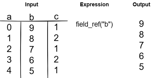
Figure 7.4 – Basic field reference expression
- Something a little tougher, Figure 7.5 shows the expression a < 4. Notice this is constructed using a compute function call named less, a field reference, and a literal value as the arguments. Because the expression is a Boolean expression, the output is a Boolean array of true or false, with each element being the corresponding result for that index in the input of column a:
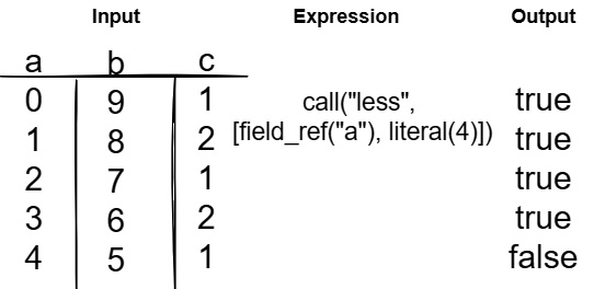
Figure 7.5 – Expression with function call and arguments
To make it easier to read and interact with, some of the most common compute functions have direct API calls for creating expressions with them. This includes your standard binary comparisons, such as less, greater, and equal, along with Boolean logic such as and, or, and not.
Using expressions for filtering data
We're going to build on the function we used for scanning the entire dataset by adding a filter to it. Let's create a new function with the same signature as the previous scan_dataset function; we can call it filter_and_select. Instead of just scanning the entire dataset like before, we're going to only read one column and then filter out some rows:
- Add these include directives to the file first. We need them for using Expression objects and compute options:
#include <arrow/compute/api.h> // general compute
#include <arrow/compute/exec/expression.h>
- For convenience, we aliased the arrow::dataset namespace to just ds previously. Now, we'll do a similar alias for the arrow::compute namespace:
namespace cp = arrow::compute;
- Our function signature is identical to the previous function, just using the new name:
std::shared_ptr<arrow::Table> filter_and_select(
const std::shared_ptr<fs::FileSystem>& filesystem,
const std::shared_ptr<ds::FileFormat>& format,
const std::string& base_dir) {
- The beginning of the function is the same for constructing the factory and dataset objects, so I won't repeat those lines here. Just do the same thing we did in the scan_dataset function. (See Step 2 under the Discovering dataset fragments section.)
- Where things change is after we create scan_builder. Instead of getting all of the columns in the dataset, we can tell the scanner to only materialize one column. In this case, we'll only retrieve column b:
auto factory = ...
auto dataset = ...
auto scan_builder = dataset->NewScan().ValueOrDie();
ABORT_ON_FAIL(scan_builder->Project({"b"}));
- Alternatively, instead of providing a list of columns, we could provide a list of expressions and names for the output columns, similar to a SQL SELECT query. The previous line would be equivalent to running SELECT b FROM dataset. This next line is the equivalent of adding a WHERE clause to the SQL query. What do you think that would look like?
ABORT_ON_FAIL(scan_builder->Filter(
cp::less(cp::field_ref("b"), cp::literal(4))));
Can you figure out what the query would look like if we were using SQL? Adding this call to Filter on the scan builder tells the scanner to use this expression to filter the data as it scans. Therefore, it's equivalent to executing something similar to this SQL query on our dataset: SELECT b FROM dataset WHERE b < 4.
- Then, just as before, we can retrieve and return a table of our results from the scan:
auto scanner = scan_builder->Finish()
.ValueOrDie();
return scanner->ToTable().ValueOrDie();
} // end of filter_and_select function
If we use the same sample dataset from back in Figure 7.5, what should our new output look like? If you run the new filter_and_select function, does it match what you'd expect? Look over the following output and double-check that your output matches!
b: int64
----
b:
[
[
3,
2,
1,
0,
]
]
Try playing around with different expressions when calling the filter function and seeing whether the output matches what you'd expect. If the filter expression references a column that isn't in the project list, the scanner still knows to read that column in addition to any it needs for the results. Next, we'll throw in some more modifications for manipulating the result columns.
Deriving and renaming columns (projecting)
Building further on our function, we can throw in some extra complexity to read the three columns, rename a column, and get a derived column using expressions. Once again, keep the same function signature and structure for the function; we're only modifying the lines that utilize scan_builder:
- First, we'll use the schema of the dataset to add a field reference for each column of the data. By getting the field list from the schema, we don't have to hardcode the whole list:
std::vector<std::string> names;
std::vector<cp::Expression> exprs;
for (const auto& field : dataset->schema()->fields()) {
names.push_back(field->name());
exprs.push_back(cp::field_ref(field->name()));
}
- Then, we add a new output column named b_as_float32, which is just the column named b casted to a 32-bit float data type. Note the structure: we are creating an expression consisting of a call to a function named cast, passing it a field reference as the only argument, and setting the options to tell it what data type it should cast to:
names.emplace_back("b_as_float32");
exprs.push_back(cp::call("cast", {cp::field_ref("b")},
cp::CastOptions::Safe(arrow::float32())));
- Next, we create another derived column named b_large, which will be a Boolean column computed by returning whether or not the value of field b is greater than 1:
names.emplace_back("b_large");
// b > 1
exprs.push_back(cp::greater(cp::field_ref("b"),
cp::literal(1)));
- Finally, we just pass the two lists of expressions and names to the scanner by calling the Project function:
ABORT_ON_FAIL(scan_builder->Project(exprs, names));
- After this, the rest of the function is identical to what it's been in the previous examples for performing the scan and retrieving the table of results.
Did you follow all of that? Can you think of what an equivalent SQL-style query would look like compared to what the code does? I mention SQL because much of the Datasets API is designed to be semantically similar to performing SQL queries on the dataset, and can even be used to implement a SQL engine!
Don't read ahead until you try it!
Seriously, try it first.
Okay, here's the answer:
SELECT
a, b, c,
FLOAT(b) AS b_as_float32,
b > 1 AS b_large
FROM
dataset
This only scratches the surface of what is possible with the Datasets and Compute APIs, but should be a useful starting point for experimentation. Play around with different types of filtering, column deriving and renaming, and so on. Maybe you have some use cases where these APIs could be used to simplify existing code. Try it out!
We've covered C++, so now, let's shift back to Python!
Using the Datasets API in Python
Before you ask: yes, the datasets API is available in Python too! Let's do a quick rundown of all the same features we just covered, but using the pyarrow Python module instead of C++. Since the majority of data scientists utilize Python for their work, it makes sense to show off how to use these APIs in Python for easy integration with existing workflows and utilities. Since Python's syntax is simpler than C++, the code is much more concise, so we can run through everything really quickly in the following sections.
Creating our sample dataset
We can start by creating a similar sample dataset to what we were using for the C++ examples with three columns, but using Python:
>>> import pyarrow as pa
>>> import pyarrow.parquet as pq
>>> import pathlib
>>> import numpy as np
>>> import os
>>> base = pathlib.Path(os.getcwd())
>>> (base / "parquet_dataset").mkdir(exist_ok=True)
>>> table = pa.table({'a': range(10), 'b': np.random.randn(10), 'c': [1, 2] * 5})>>> pq.write_table(table.slice(0, 5), base / "parquet_dataset/data1.parquet")
>>> pq.write_table(table.slice(5, 10), base / "parquet_dataset/data2.parquet")
After we've got our imports squared away and set up a path to write the Parquet files to, the highlighted lines are where we actually construct the sample dataset. We create a table with 10 rows and 3 columns, then split the table into 2 Parquet files that each have 5 rows in them. Using the Python pathlib library makes the code very portable since it will handle the proper formatting of file paths based on the operating system you're running it under.
Discovering the dataset
Just like with the C++ library, the dataset library for Python is able to perform a discovery of file fragments by passing the base directory to start searching from. Alternatively, you could pass the path of a single file or a list of file paths instead of a base directory to search:
>>> import pyarrow.dataset as ds
>>> dataset = ds.dataset(base / "parquet_dataset", format="parquet")
>>> dataset.files
['<path>/parquet_dataset/data1.parquet', '<path>/parquet_dataset/data2.parquet']
<path> should be replaced by the path to the directory you created for the sample dataset in the previous section.
This will also infer the schema of the dataset just like the C++ library. By default, it will do this by reading the first file in the dataset. You could also manually supply a schema to use as an argument to the dataset function instead:
>>> print(dataset.schema.to_string(show_field_metadata=False))
a: int64
b: double
c: int64
Finally, we also have a method to load the entire dataset (or a portion of it) into an Arrow table just like the ToTable method in C++:
>>> dataset.to_table()
pyarrow.Table
a: int64
b: double
c: int64
----
a: [[0,1,2,3,4],[5,6,7,8,9]]
b: [[[[0.4496826452924734,0.8187826910251114,0.293394262192757,-0.9355403104276471,-0.19315460805569024],[1.3384156936773497,-0.6000310181068441,0.16303489615416472,-1.4502901450565746,-0.5973093999335979]]
c: [[1,2,1,2,1],[2,1,2,1,2]]
While we used Parquet files for the preceding examples, the dataset module does allow specifying the file format of your dataset during discovery.
Using different file formats
Currently, the Python version supports the following formats, providing a consistent interface regardless of the underlying data file format:
- Parquet
- ORC
- Feather/Arrow IPC
- CSV
More file formats are planned to be supported over time. The format keyword argument to the dataset function allows specifying the format of the data.
Filtering and projecting columns with Python
Like the C++ interface, the pyarrow library provides an Expression object type for configuring filters and projections of the data columns. These can be passed to the dataset as arguments to the to_table function. For convenience, operator overloads and helper functions are provided to help with constructing filters and expressions. Let's give it a try:
- Selecting a subset of columns for the dataset will only read the columns requested from the files:
>>> dataset.to_table(columns=['a', 'c'])
pyarrow.Table
a: int64
c: int64
----
a: [[0,1,2,3,4],[5,6,7,8,9]]
c: [[1,2,1,2,1],[2,1,2,1,2]]
- The filter keyword argument can take a Boolean expression that defines a predicate to match rows against. Any row that doesn't match will be excluded from the returned data. Using the field helper function allows specifying any column in the table, regardless of whether or not it's a partition column or in the list of projected columns:
>>> dataset.to_table(columns=['a', 'b'], filter=ds.field('c') == 2)
pyarrow.Table
a: int64
b: double
----
a: [[1,3],[5,7,9]]
b: [[0.8187826910251114,-0.9355403104276471],[1.3384156936773497,0.16303489615416472,-0.5973093999335979]]
- You can also use function calls and Boolean combinations with the expressions to create complex filters and perform set membership testing:
>>> dataset.to_table(filter=(ds.field('a') > ds.field('b')) & (ds.field('a').isin([4,5])))
pyarrow.Table
a: int64
b: double
c: int64
----
a: [[4],[5]]
b: [[-0.19315460805569024],[1.3384156936773497]]
c: [[1],[2]]
- Column projection can be defined using expressions by passing a Python dictionary that maps column names to the expressions to execute for deriving columns:
>>> projection = {
... 'a_renamed': ds.field('a'),
... 'b_as_float32': ds.field('b').cast('float32'),
... 'c_1': ds.field('c') == 1,
... }
>>> dataset.to_table(columns=projection)
pyarrow.Table
a_renamed: int64
b_as_float32: float
c_1: bool
----
a_renamed: [[0,1,2,3,4],[5,6,7,8,9]]
b_as_float32: [[0.44968265,0.8187827,0.29339427,-0.9355403,-0.1931546],[1.3384157,-0.600031,0.1630349,-1.4502902,-0.5973094]]
c_1: [[true,false,true,false,true],[false,true,false,true,false]]
All of the examples so far have involved reading the entire dataset and performing the projections or filters, but we wanted to be able to handle very large datasets that potentially won't fit in memory, right? Both the C++ and Python dataset APIs support streaming, iterative reads for these types of workflows, and allowing processing of data without loading the entire dataset at once. We're going to cover working with the streaming APIs next.
Streaming results
You'll recall from the beginning of this chapter, in the Querying multifile datasets section, that I mentioned this was the solution for when you had multiple files and the dataset was potentially too large to fit in memory all at one time. So far, the examples we've seen used the ToTable function to completely materialize the results in memory as a single Arrow table. If your results are too large to fit into memory all at one time, this obviously won't work. Even if your results could fit into memory, it's not the most efficient way to perform the query anyway. In addition to the ToTable (C++) or to_table (Python) function we've been calling, the scanner also exposes functions that return iterators for streaming record batches from the query.
To demonstrate the streaming, let's use a public AWS S3 bucket hosted by Ursa Labs, which contains about 10 years of NYC taxi trip record data in Parquet format. The URI for the dataset is s3://ursa-labs-taxi-data/. Even in Parquet format, the total size of the data there is around 37 GB, significantly larger than the memory available on most people's computers. We're going to play around with this dataset with both C++ and Python, so let's have some fun!
First, let's see how many files and rows are in this very large dataset. We'll try Python first. Let's use Jupyter or IPython so that we can time the operations using %time:
In [0]: import pyarrow.dataset as ds
In [1]: %%time
...: dataset = ds.dataset('s3://ursa-labs-taxi-data/')...: print(len(dataset.files))
...: print(len(dataset.count_rows())
...:
...:
125
1547741381
Wall Time: 5.63 s
Using the Python dataset library, we can see that there are 125 files in that dataset and were able to count the number of rows (over 1.5 billion) across those 37 gigabytes of 125 files in around 5.6 seconds. Not bad, not bad. Now, using C++, first we'll time the dataset discovery in finding all the files. Let's get the include directives out of the way first:
#include <arrow/filesystem/api.h>
#include <arrow/dataset/api.h>
#include "timer.h" // located in this book's GitHub Repository
#include <memory>
#include <iostream>
Then, we have the namespace aliases for convenience:
namespace fs = arrow::fs;
namespace ds = arrow::dataset;
Before we can utilize the interfaces for S3, we need to initialize the AWS S3 libraries by calling the aptly named InitializeS3 function:
fs::InitializeS3(fs::S3GlobalOptions{});auto opts = fs::S3Options::Anonymous();
opts.region = "us-east-2";
Working with S3FileSystem works just like using the local filesystem in the previous examples, making this really easy to work with:
std::shared_ptr<ds::FileFormat> format =
std::make_shared<ds::ParquetFileFormat>();
std::shared_ptr<fs::FileSystem> filesystem =
fs::S3FileSystem::Make(opts).ValueOrDie();
fs::FileSelector selector;
selector.base_dir = "ursa-labs-taxi-data";
selector.recursive = true; // check all the subdirectories
By setting the recursive flag to true, the discovery mechanisms of the Datasets API will properly iterate through the keys in the S3 bucket and find the various Parquet files. Let's create our dataset and time how long it takes:
std::shared_ptr<ds::DatasetFactory> factory;
std::shared_ptr<ds::Dataset> dataset;
{timer t; // see timer.h,
// will print elapsed time on destruction
factory =
ds::FileSystemDatasetFactory::Make(filesystem,
selector, format,
ds::FileSystemFactoryOptions()).ValueOrDie();
dataset = factory->Finish().ValueOrDie();
}
Remember, the handy timer object you see in the code snippet will output the amount of time between its construction and when it goes out of scope, writing directly to the terminal. Compiling and running this code shows, in the output, that it took 1,518 milliseconds to discover the 125 files of the dataset. Then, we can add a call to count the rows, as we did in Python:
auto scan_builder = dataset->NewScan().ValueOrDie();
auto scanner = scan_builder->Finish().ValueOrDie();
{timer t;
std::cout << scanner->CountRows().ValueOrDie()
<< std::endl;
}
We get the same 1.54-billion-row count, only this time it took just 2,970 milliseconds, or 2.9 seconds, compared to the 5.6 seconds that Python took. Granted, this is an easy one. It just needs to check the metadata in each Parquet file for the number of rows in it and then sum them all together. The amount of data it needs to read is actually very little.
Let's try something a bit more interesting than just listing the total number of rows. How about getting the average number of passengers across the entire dataset? OK, it's not a complex expression to compute. But the point is to show how easy it is to do something like this and how quickly it can execute. How long do you think it would take to perform this computation across the entire dataset using just my laptop? No compute cluster or anything, just a single laptop on my home network. Remember, this isn't just a simple "calculate the mean of a column." Look at Figure 7.6, a visual representation of what we're going to do. It's basically a pipeline:
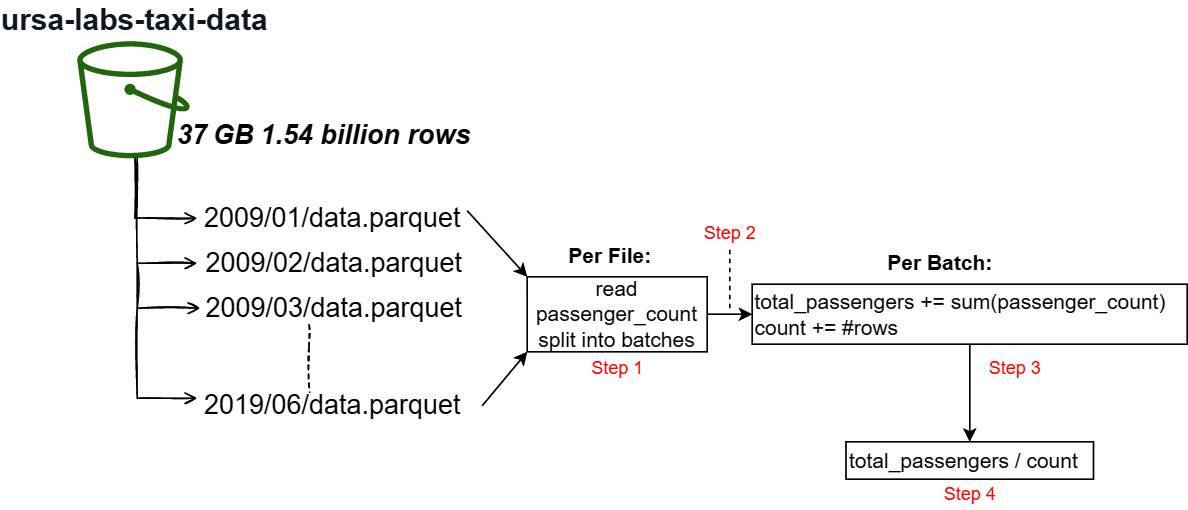
Figure 7.6 – Dataset accumulation
Let's go through this step by step:
- The dataset scanner will read only the passenger_count column from each file asynchronously and split the data into configurable batches.
- The batches will be streamed so that we never load the entire dataset in memory at one time.
- For each batch we get in the stream, we'll use the compute library to calculate the sum of the data and add it to a running total. We'll also keep track of the total number of rows we see.
- Once there are no more batches, we can just compute the mean using the values we computed.
How complex do you think this will be to write? How long do you think it'll take to run? Ready to be surprised?
First, we'll do it in Python using the dataset object we created earlier:
In [2]: import pyarrow.compute as pc
In [3]: scanner = dataset.scanner(columns=['passenger_count'], use_async=True)
In [4]: total_passengers = 0
In [5]: total_count = 0
In [6]: %%time
...: for batch in scanner.to_batches():
...: passengers += pc.sum(batch.column('passenger_count')).as_py()...: count += batch.num_rows
...: mean = passengers/count
...:
...:
Wall time: 2min 37s
In [7]: mean
1.669097621032076
Simple enough! And it only took around 2.5 minutes to run on a single laptop, to calculate the mean across over 1.5 billion rows. Not bad, if I say so myself. After a bit of testing, it turns out that the bottleneck here is the connection with S3 to transfer the gigabytes of data being requested across the network, rather than the computation.
Anyway, now the C++ version. It's just a matter of using a different function on the scanner object. Creating the factory and the dataset objects works the same as in all the previous C++ examples, so let's create our scanner:
#include <atomic> // new header
...
// creating the factory and dataset is the same as before
{timer t;
auto scan_builder = dataset->NewScan().ValueOrDie();
scan_builder->BatchSize(1 << 28); // default is 1 << 20
scan_builder->UseThreads(true);
scan_builder->Project({"passenger_count"});auto scanner = scan_builder->Finish().ValueOrDie();
With our scanner all set up, we then pass a lambda function to the Scan method of the scanner, which will asynchronously call it as record batches are received. Because this is done in a thread pool, potentially at the same time, we use std::atomic<int64_t> to avoid any race conditions:
std::atomic<int64_t> passengers(0), count(0);
ABORT_ON_FAIL(scanner->Scan(
[&](ds::TaggedRecordBatch batch) -> arrow::Status {ARROW_ASSIGN_OR_RAISE(auto result,
cp::Sum(batch.record_batch->
GetColumnByName("passenger_count")));passengers +=
result.scalar_as<arrow::Int64Scalar>().value;
count += batch.record_batch->num_rows();
return arrow::Status::OK();
}));
If we look back at the Python version we wrote, you might be wondering why we didn't need any synchronization there. This is because scanner.to_batches is a Python generator producing a stream of record batches. There's never the potential that we're processing more than one record batch at a time. In the preceding C++ code snippet, we pass a callback lambda to the scanner, which can potentially call it from multiple threads simultaneously. With this multithreaded approach, and the potential that we might process more than one record batch simultaneously, std::atomic ensures that everything is processed correctly.
Finally, we can just calculate our result and output it once the scan has completed:
double mean =
double(passengers.load())
/ double(count.load());
std::cout << mean << std::endl;
} // end of the timer block
Running this locally on my laptop, it runs on average for about 1 minute and 53 seconds, or roughly 26% faster than the Python version.
If you look back at Figure 7.6, you'll see the structure of the keys in the AWS S3 bucket and how they are partitioned into folders by year and month. Well, we can take advantage of that to super-charge any filtering we want to do by those fields! All you have to do is use the partitioning settings that are included with the Arrow Datasets API, which is, of course, the next thing we're going to do.
Working with partitioned datasets
In the previous example, we shifted from files in a flat directory to files that were partitioned into directories. If we were to place filter expressions into the scanner, it would have to open up each file and potentially read the whole file first, and then filter the data. By organizing the data into partitioned, nested subdirectories, we can define a partitioning layout where the names of the subdirectories provide information about which subset of the data is stored there. Doing this allows us to completely skip loading files that we know won't match a filter.
Let's look at the partitioning structure used by the taxi dataset on S3 again:
2009/
01/data.parquet
02/data.parquet
...
2010/
01/data.parquet
02/data.parquet
...
...
It may be obvious, but using this structure means that we can assume by convention that the file located at 2009/01/data.parquet will only contain data where year == 2009 and month == 1. By using the configurations, we can even provide pseudo-columns for our data that represent the year and month, even though those columns don't exist in the files. Let's give it a try, first in C++, initializing the S3 filesystem and creating the selector object as before:
ds::FileSystemFactoryOptions options;
options.partitioning =
ds::DirectoryPartitioning::MakeFactory({"year", "month"});auto factory = ds::FileSystemDatasetFactory::Make(
filesystem, selector, format, options).ValueOrDie();
auto dataset = factory->Finish().ValueOrDie();
auto fragments = dataset->GetFragments().ValueOrDie();
for (const auto& fragment : fragments) {std::cout << "Found Fragment: "
<< (*fragment)->ToString() << std::endl;
std::cout << "Partition Expression: "
<< (*fragment)->partition_expression().ToString()
<< std::endl;
}
The highlighted lines are the additions made as compared to the way we constructed the dataset in the previous examples. The DirectoryPartitioning factory object is used to add the partitioning option to the factory denoting the order of the pieces of the file paths and what they should be called. This even adds columns to the schema of the created dataset named year and month, inferring the types of those columns from the values. If we print out the schema, we can confirm this; just add a line to print out the schema:
std::cout << dataset->schema()->ToString() << std::endl;
We see it reflected in the output:
vendor_id: string
...
year: int32
month: int32
In this case, the dataset inferred from the values that our year and month columns were 32-bit integer fields. If you prefer, you could instead specify the types directly with the partitioning options by providing a full Arrow schema object:
options.partitioning = std::make_shared<ds::DirectoryPartitioning>(
arrow::schema({arrow::field("year", arrow::uint16()), arrow::field("month", arrow::int8())}));
Of course, we can do exactly the same thing with Python, like so:
In [3]: part = ds.partitioning(field_names=["year", "month"])
In [4]: part = ds.partitioning(pa.schema([("year", pa.uint16()), ("month", pa.int8())])) # or specify the typesIn [5]: dataset = ds.dataset('s3://ursa-labs-taxi-data/', partitioning=part, format='parquet')In [6]: for fragment in dataset.get_fragments():
...: print("Found Fragment:", fragment.path) ...: print("Partition Expression:", fragment.partition_expression)...:
In both cases, C++ or Python, our code snippets provide the same output list of files and partition expressions:
Found Fragment: ursa-labs-taxi-data/2009/01/data.parquet
Partition Expression: ((year == 2009) and (month == 1))
Found Fragment: ursa-labs-taxi-data/2009/02/data.parquet
Partition Expression: ((year == 2009) and (month == 2))
...
A common partitioning scheme that is frequently seen is the partitioning scheme used by Apache Hive, a SQL-like interface for files and data that integrates with Hadoop. The Hive partitioning scheme includes the name of the field in the path along with the value, instead of just the value. For example, with the taxi data we were just using, instead of a file path of /2009/01/data.parquet, it would be /year=2009/month=1/data.parquet. Because this scheme is very common due to the proliferation and use of Apache Hive, the Arrow library already provides convenient classes for specifying the Hive partition scheme, regardless of whether you're using C++, as follows:
options.partitioning = ds::HivePartitioning::MakeFactory();
// or specify the schema to define the types
options.partitioning = std::make_shared<ds::HivePartitioning>(
arrow::schema({arrow::field("year", arrow::uint16()), arrow::field("month", arrow::int8())}));
Or if you're using Python, as follows:
In [7]: dataset = ds.dataset('s3://ursa-labs-taxi-data/', partitioning='hive', format='parquet') # infer the typesIn [8]: part = ds.partitioning( # or specify the schema
...: pa.schema([("year", pa.uint16()), ("month", pa.int8())]),...: flavor='hive') # and denote it is using the hive style
If we scan the dataset after defining the partitioning using a filter on either or both of the fields that we partition on, we won't even read the files whose partition expressions don't match the filter. We can confirm that by using filters and checking how long things take. Let's count the rows based on a filter so we can confirm this:
In [9]: dataset = ds.dataset('s3://ursa-labs-taxi-data', partitioning=part, format='parquet')In [10]: %time dataset.count_rows(filter=ds.field('year') == 2012)Wall time: 421 ms
Out[10]: 178544324
In [11]: import datetime
In [12]: start = pa.scalar(datetime.datetime(2012, 1, 1, 0, 0, 0))
In [13]: end = pa.scalar(datetime.datetime(2013, 1, 1, 0, 0, 0))
In [14]: %%time
... : dataset.count_rows(filter=
... : (ds.field('pickup_at') >= start) & ... : (ds.field('pickup_at') < end))... :
... :
Wall time 20.9 s
Out[14]: 178544324
In the first highlighted section, we count the number of rows that meet the filter where the year field is equal to the value 2012. This turns out to be very quick and easy despite the size of the dataset because of the partitioning. We just need to read the Parquet metadata of each file under the 2012 directory and its subdirectories and add up the number of rows in each one, taking only 421 milliseconds.
In the second highlighted section, we use two timestamp scalar values to create a filter expression. We then count the rows where the pickup_at field is greater than or equal to January 1, 2012, and less than January 1, 2013. Because it's not a partition field, we have to open and read every file in the dataset to check the rows to find out what rows match the filter. Granted, because Parquet files can maintain statistics on their columns, such as the minimum and maximum value, this isn't as expensive as having to check every single last row. We don't have to read all 1.5 billion rows to get the answer but can instead use the statistics to skip large groups of rows. Unfortunately, this still means we have to at least read the metadata from every single file in the dataset, instead of being able to skip files entirely as we did with the partition field. That extra work leads to the almost 21 seconds it takes to get the same answer, almost 49 times slower than using the partition field.
Try doing the same experiment with the C++ library!
Now, that's all fine and helpful when reading data, but what about when you have to write data? The Datasets API also simplifies writing data, even partitioning it for you if you desire.
Writing partitioned data
There are two sides to working with data: querying data that exists and writing new data. Both are heavily important workflows and so we want to simplify both. In the previous sections, we were looking solely at reading and querying a dataset that existed. Writing a dataset is just as easy as writing a single table. (Remember? We did that back in Chapter 2, Working with Key Arrow Specifications.)
If you have a table or record batch already in memory, then you can easily write your dataset. Instead of providing a filename, you provide a directory and a template for what the files will get named. As usual, Python has a simpler syntax for you to use. Have a look:
In [15]: base = pathlib.Path(...) # use base path for your datasets
In [16]: root = base / "sample_dataset"
In [17]: root.mkdir(exit_ok=True)
In [18]: ds.write_dataset(table, root, format='parquet')
This will write a single file named part-0.parquet to the directory specified. If you want to name it differently, then you can pass the basename_template keyword argument with a string describing the template for the filenames. The syntax for this template is pretty simple; it's just a string containing {i} in it. The {i} characters will be replaced by an integer that will increment automatically as files get written based on the other options, such as the partition configuration and maximum file sizes. The write_dataset function will automatically partition data for you if you pass the same partitioning option as we did for reading:
In [19]: part = ds.partitioning(pa.schema([('foobar', pa.int16())]),... : flavor='hive')
In [20]: ds.write_dataset(table, root, format='parquet',
... : partitioning=part)
It will automatically create directories for the partitions and write the data, accordingly, using the same basename_template option that can be passed when writing a single table to name the individual files of each partition. All of this functionality is, of course, also available from the C++ library:
auto dataset = std::make_shared<ds::InMemoryDataset>(table);
auto scanner_builder = dataset->NewScan().ValueOrDie();
auto scanner = scanner_builder->Finish().ValueOrDie();
auto format = std::make_shared<ds::ParquetFileFormat>();
ds::FileSystemDatasetWriteOptions write_opts;
write_opts.file_write_options = format->DefaultWriteOptions();
write_opts.filesystem = filesystem;
write_opts.base_dir = base_path;
write_opts.partitioning = std::make_shared<ds::HivePartitioning>(
arrow::schema({arrow::field("year", arrow::uint16()), arrow::field("month", arrow::int8())}));
write_opts.basename_template = "part{i}.parquet";ABORT_ON_FAIL(ds::FileSystemDataset::Write(write_opts, scanner));
Did you notice that the Write function takes a scanner? Can you think of why that might be the case?
We're talking about potentially very large datasets, larger than can fit into memory at one time. Because the Write function takes scanner as a parameter, you can very easily stream data to the writer from a scanner. That scanner could be configured using filters and projection to customize the record batch stream that you're writing. The Python version of the dataset writer can also take a scanner as the first argument instead of a table.
We can also write our dataset in different formats than just Parquet and combine it with filtering our data. For example, we could write out a portion of the taxi dataset as CSV files with just the following code changes from the previous example.
Just like before, we call fs::InitializeS3 and create FilesystemDatasetFactory with the partition options, file selector, and format. However, this time we're going to add some options to control how it infers the schema. We mentioned InspectOptions back in the Discovering dataset fragments section, talking about discovering the schema. By default, the factory will only read one fragment to determine the schema of the dataset.
At the start of this Working with partitioned datasets section, we printed out the schema to see the addition of the year and month fields. If you run that code snippet again, take note of the type of the field named rate_code_id:
...
rate_code_id: null
...
This is the schema that was inferred by only reading the first fragment. Now, let's add the necessary options to inspect all the fragments and validate the schemas by adding the highlighted lines:
auto factory = ds::FileSystemDatasetFactory::Make(
filesystem, selector,
format, options).ValueOrDie();
ds::FinishOptions finish_options;
finish_options.validate_fragments = true;
finish_options.inspect_options.fragments =
ds::InspectOptions::kInspectAllFragments;
auto dataset = factory->Finish(finish_options);
By setting the options to both inspect all the fragments and validate them, the factory will compose a common schema if it is possible. When we now print out the dataset's schema, note the rate_code_id field again:
...
rate_code_id: string
...
DatasetFactory inspected all the fragments and created a combined schema. Some of the fragments have the rate_code_id field as type null, and others have it as type string. Since we can trivially cast from a null type to a string array consisting of only null values, it's a valid combined schema to identify it as a string column. If you tried processing this dataset in its entirety before this, you may have encountered an error that looks like this:
Unsupported cast from string to null using function cast_null
This makes sense if you think about it. If our dataset's schema has a null type for the column, when we encounter a fragment with type string for this column, it attempts to cast the values. While we can easily cast a null array to a string array consisting entirely of null values, it's invalid to do the reverse: casting a string array with values to a null array. By taking the time to inspect our fragments and generate the combined schema, we fix this problem! Now, to write our data out as CSV files, all we need to do is use CsvFileFormat:
auto format = std::make_shared<ds::CsvFileFormat>();
ds::FileSystemDatasetWriteOptions write_opts;
auto csv_write_options =
std::static_pointer_cast<ds::CsvFileWriteOptions>(
format->DefaultWriteOptions());
csv_write_options->write_options->delimiter = '|';
write_opts.file_write_options = csv_write_options;
...
ABORT_ON_FAIL(ds::FileSystemDataset::Write(write_opts, scanner));
Note the highlighted lines. After we create our default options using the CsvFileFormat class, we can set various options, such as the delimiter to use when writing. In this case, we write our data as pipe-delimited files. The same holds true for using IpcFileFormat or OrcFileFormat to write data in those respective data formats.
An Exercise for You
Write a function that repartitions a large dataset without pulling the entirety of the data into memory at one time. Try it in C++ and/or in Python to familiarize yourself with writing datasets. Play around with the batch sizes and other options to see how you can tweak it for performance.
Finally, the dataset writer also provides hooks that can be customized to allow inspecting and customizing the files that are written. In Python, you can provide a file_visitor function that takes in the written file as an argument to the write_dataset function. In C++, the FileSystemDatasetWriteOptions object has two members, writer_pre_finish and writer_post_finish, which are each a lambda function that takes a pointer to FileWriter and is called before and after each FileWriter finalizes a file.
Another Exercise for You to Try
Try writing a partitioned dataset and constructing an index of the files written and some metadata about them using the exposed write hooks via the file_visitor or writer_pre_finish/writer_post_finish functions.
There's a wealth of options that exist for datasets, ranging from the different file formats to using UnionDataset to interact with multiple physical datasets compiled into one interface. You can also manipulate the file format objects to set format-specific options for your reads and writes. Whether you're reading, writing, or using partitioned or non-partitioned data, the Datasets API is an extremely useful building block for many use cases. It's also particularly nice for ad hoc exploration of very large datasets, providing a huge amount of flexibility in how you can choose to interact with it and combine it with the Compute API and other Arrow usage. Go try out combining different ways of computing and manipulating data in huge datasets using these APIs before you move on. Seriously, do it! It's fun!
Summary
By composing these various pieces together (the C Data API, Compute API, and Datasets API), and gluing infrastructure on top, anyone should be able to create a rudimentary query and analysis engine that is fairly performant right away. The functionality provided allows for abstracting away a lot of the tedious work for interacting with different file formats and handling different location sources of data, to provide a single interface that allows you to get right to work in building the specific logic you need. Once again, it's the fact that all these things are built on top of Arrow as an underlying format, which is particularly efficient for these operations, that allows them to all be so easily interoperable.
So, where do we go from here?
Well, you might remember in Chapter 3, Data Science with Apache Arrow, when discussing Open Database Connectivity (ODBC), I alluded to the idea of something that might be able to replace ODBC and JDBC as universal protocols for interacting with databases. Armed with everything you've learned so far, we're going to look at building distributed systems using Apache Arrow next.
The next chapter is Chapter 8, Exploring Apache Arrow Flight RPC. The Arrow Flight protocol is a highly efficient way to pass data across the network, utilizing Arrow's IPC format as the primary data format. Over the course of the next chapter, we're going to build a Flight server and client for passing data back and forth in a customizable way. Hold on to your keyboards, this is going to be fun…
OK, well at least I think it's fun. Hopefully, you do too!