
Chapter 3: Data Science with Apache Arrow
So far, we've covered the Apache Arrow format and how to read various types of data from local disks or cloud storage into Arrow-formatted memory, but if you aren't the one actually building tools and utilities for others to use, then what does this mean for you? You'll be able to benefit from things that people will build using Arrow, such as new fancy libraries, performance enhancements, and utilities. But, how can you materially change your workflow to get some of these improvements right now? That's what we're going to be covering in this chapter, specific examples of Arrow enhancing existing data science workflows and enabling new ones.
In this chapter, we'll look at the following topics:
- How Open Database Connectivity (ODBC) is being improved upon and will eventually, hopefully, be rendered obsolete by Arrow communication protocols
- Leveraging the topics we covered in the previous chapters with Apache Spark and Jupyter notebooks
- Usage of Perspective, an interactive analytics and data visualization component for web and Python/JupyterLab
- An example of a full stack application using Arrow as its internal data format
Technical requirements
With the exception of the last section of the chapter, this chapter is more focused on specific examples rather than code snippets, but if you want to try performing the same tests as the examples, you'll need the following:
- An internet-connected computer.
- A single- or multiple-node Apache Spark cluster also running Jupyter. Docker is the easiest way to set this up, which is what we'll use in this chapter.
Let's begin!
ODBC takes an Arrow to the knee
Open Database Connectivity (ODBC) is a standardized Application Programming Interface (API) for accessing databases originally designed and built in the early 1990s. The development of ODBC intended to enable applications to be independent of their underlying database by having a standardized API to use that would be implemented by database-specific drivers. This allowed a developer to write their application and potentially easily migrate to a different database by simply specifying a different driver. In 1997, the Java Database Connectivity (JDBC) API was developed to provide a common API for Java programs to manage multiple drivers and connect either by bridging to an ODBC connection or by other types of connections, which all have different pros and cons. Almost 30 years later, these technologies are still the de facto standard way to communicate with Structured Query Language (SQL) databases.
That all being said, computing, and data in particular, have changed significantly in that time frame. Back then, computers didn't have the dozens of cores that they have today, and systems were much more monolithic. Big data's rise, alongside the increase in distributed systems and the emergence of data science as a full profession, has shown the cracks in the promises of performance and scalability from ODBC and JDBC. Unfortunately, it's going to take a while for everything to follow suit to new technologies, so there needs to be a stepping-stone, an intermediate step, to help push things towards leveraging new technologies such as Arrow.
In the context of data science, most will interact with ODBC or JDBC when working with loading data for analysis into scripts or tools. Business intelligence (BI) utilities nearly universally accept ODBC and JDBC interfaces as their primary way to interact with data sources. It makes sense, as they only have to implement their code once in terms of the ODBC standard and that gives them access to any data source that publishes an ODBC driver. Some of the big names in this space would be tools such as Tableau and Power BI, both of which support ODBC data source access. Supporting native Arrow data, Parquet files, and other communications would mean faster data access, quicker computations, and snappier interactive dashboards for users. How does it do that? Well, by reducing and eliminating the translations and copies of data being made at every level through direct support of Arrow in all stages. We've already mentioned in Chapter 2, Working with Key Arrow Specifications, one such example: the Arrow-JDBC adapter.
Lost in translation
Even when systems speak the same standard protocol, there might be a whole bunch of translations and copies happening under the hood. ODBC, for all its benefits, was still designed during a time when it was much more common to be requesting wide tables with large numbers of columns and fewer rows as compared to modern data analysis. While it enabled connectivity between different disparate systems, there's still a lot of translating and copying that has to happen in the ODBC drivers for everything to work correctly. Figure 3.1 shows a comparison between a standard data science workflow using typical ODBC or JDBC and using the Arrow-JDBC adapter.
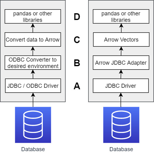
cLook first at the left side of Figure 3.1, the typical case when using JDBC. There are three points where data has to be translated between formats, as follows:
- First, data is translated inside the JDBC/ODBC driver from whatever format the database speaks natively into the JDBC/ODBC standards.
- Next, data has to be translated into the necessary objects/memory for your choice of programming language/environment. For example, if you're using Python and pandas, you have to either use ODBC or Python-native drivers (lower performance) or a JDBC driver, which then has to convert the JDBC objects to Python objects, and this has a high cost.
- Finally, however you got your data into your environment, if the interface didn't spit out Arrow data objects, then once again there's a translation to Arrow before you can finally interact with the data in pandas. (Sure, you can go straight to pandas, but we've already shown that the creation of pandas from Arrow has a negligible cost, so it doesn't save you anything.)
Compare this with the workflow on the right side of Figure 3.1:
- If the underlying database doesn't speak Arrow natively, there's a translation from the database data into JDBC objects.
- The Arrow-JDBC adapter will then convert the JDBC objects directly into Arrow vectors in memory that is not managed by the Java Virtual Machine (JVM).
- The addresses of the vectors can be passed directly into Python, which can then reference the memory exactly where it is (as shown in Chapter 2, Working with Key Arrow Specifications) rather than having to translate or copy the data.
By reducing the translations and copies, we reduce the CPU usage, memory usage, and run time. In short, it goes much faster and requires fewer resources! This could apply directly to tools such as Tableau and Power BI if they supported Arrow natively. We're starting to see this happen as more and more companies start enabling Arrow data as the memory format for ODBC and JDBC drivers. Here's a short list of a couple of tools and companies that have already built support for Arrow into their clients, drivers, and connectors:
- Snowflake updated their ODBC drivers and Python client to convert their internal memory format to Arrow for data transfer and saw between 5x and 10x performance improvements depending on the use case (https://www.snowflake.com/blog/fetching-query-results-from-snowflake-just-got-a-lot-faster-with-apache-arrow/).
- Google's BigQuery added support for pulling data using Arrow record batches and users saw from 15x to 31x performance improvements for retrieving data into pandas DataFrames from the BigQuery Storage API (https://medium.com/google-cloud/announcing-google-cloud-bigquery-version-1-17-0-1fc428512171).
- Dremio Sonar's JDBC and ODBC drivers have always utilized Arrow to transfer data to users and since Arrow is Dremio Sonar's internal memory format (unlike BigQuery and Snowflake). There is zero data conversion from when the data is read to when the result set is returned to the client.
This is, of course, not a full list, just what I was able to find easily or am already using myself. I'm sure that by the time this book is in your hands, there will likely be even wider support. But, eventually, we may see ODBC and JDBC as a protocol replaced by something better. (Yes, I'm alluding to something but you'll have to keep reading to find out what!)
With ODBC/JDBC as the primary connector used to retrieve data, the other big heavyweight in the data science space is Apache Spark, combined with the Jupyter Notebook, which is one of the most common distributed computing platforms used by data scientists. Even if they aren't using it directly, Spark also is the underlying technology of (or used by) a large number of commercial products such as AWS Glue, Cloudera, and Databricks. Adding Arrow support to Spark at a low level, in conjunction with Parquet files, has resulted in enormous performance gains that are easy to replicate and show off. Follow along!
SPARKing new ideas on Jupyter
Apache Spark is an open source analytics engine for distributed processing across large clusters to take advantage of parallelism and fault tolerance that can come from such designs. It is also very likely, in my opinion, the most loved and simultaneously hated piece of software since the invention of JavaScript! The love comes from the workflows it enables, but it is notoriously fragile and difficult to use properly. If you aren't familiar with Spark, it is commonly used in conjunction with Scala, Java, Python, and/or R in addition to being able to run distributed SQL queries. Because Python is easy to pick up and very quick to write, data scientists will often utilize Jupyter notebooks and Python to quickly create and test models for analysis.
This workflow is excellent for quickly iterating on various ideas and proving their correctness. However, engineers and data scientists often find themselves beholden by the fact that, frankly, Python is pretty slow. In addition, unless you have access to a large cluster with a huge number of cores, Spark can also be fairly slow depending on the calculations and use case. That brings us to the question of how we can simultaneously make it easier to write code for the calculations we want, and improve the performance of those calculations. The answer is integration with Arrow and Parquet and taking advantage of columnar formats.
Understanding the integration
First thing's first, I should point out that this isn't a case of Spark versus Arrow, but rather where Arrow can be used to enhance existing Spark pipelines. Many Apache Spark pipelines would never need to use Arrow, and Spark has its own in-memory DataFrame format that is distinct from Arrow's. Converting between the two would introduce a performance drop, so any benefits need to be considered and weighed against this. With all of that said, where this marriage works beautifully is when it comes to switching your pipelines and data to different languages and libraries, such as when you use a pandas user-defined function as part of your Spark pipeline. In this situation, Spark can utilize Arrow for performing the conversion and communication for the benefits we saw in the last chapter when converting. Figure 3.2 can help explain this a bit more by showing a simplified representation of how PySpark works.
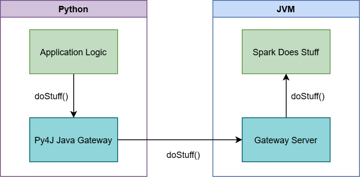
Figure 3.2 – PySpark Using Py4J to communicate
When you run PySpark, two processes are started up for you, the Python interpreter itself and a JVM process. This is because Spark is written using Scala/Java, not Python. All the heavy lifting that Spark does is actually done outside of the Python process, with Python providing an interface to send commands to Spark via the Py4J bridge. The problem is that when you want to interact with the data in Python, then send it to Spark, and then get the results back, you need to send the data across this bridge somehow. Imagine loading a 4 GB pandas DataFrame in Python, manipulating it a bit, and then sending it to Spark for computations and further analysis. Figure 3.3 shows what happens under the hood:
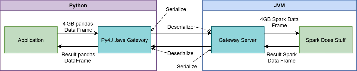
Figure 3.3 – Sending data back and forth to Spark from PySpark
In Figure 3.3, you can see that the 4 GB of data will need to get serialized somehow into a stream of bytes, passed to the JVM process to get deserialized so Spark can operate on it, only for the results from Spark to go through the same process in reverse. When you're dealing with large datasets, optimizing this passing of the data can save you a ton of time and computing resources! Also, keep in mind that since pandas DataFrames and Spark DataFrames are different formats, there's still a conversion to be done there as well. This is where Arrow can come in and speed things up.
Essentially, any time you want to use a library that isn't using Spark's native in-memory format, you are going to have to do a translation between those formats. This includes some Java libraries and any non-Java library (such as running Python user-defined functions). There are some operations that are faster with Arrow's format than with Spark's, and vice versa, but in most cases, it's only worth it if you are doing a lot of work in a non-Spark format such as pandas, which happens frequently concerning data scientists since pandas is a lot more friendly and easy to use than Spark itself.
In this example, we're going to use a slice of one of the files from the free and open NYC Taxi dataset, which is included in the sample_data folder of the GitHub repository that accompanies this book, which we've used before (such as with the exercises at the end of Chapter 1, Getting Started with Apache Arrow). I've intentionally only grabbed a slice of the file instead of the entire thing since this is to showcase examples that will be easy to run and replicate using Docker rather than needing your own Spark cluster. There are two main use cases we're going to look at:
- Getting the data into and out of Spark from the raw CSV file
- Performing a normalization calculation on one or more numeric fields in the dataset
Before we dive into the code first, let's spin up our development environment with Docker.
Everyone gets a containerized development environment!
Instead of fiddling with installing Apache Spark and Jupyter ourselves, we can launch a consistent and useful development environment using Docker. No manually dealing with dependencies, just an easy-to-share image name and you can replicate the examples. Oh, Docker. How much do we love you? Let us count the ways!
- The Docker Hub community provides pre-packaged development environment containers that are easy to test and use.
- We don't have to fight and figure out the proper way to install Spark and all of its dependencies; just use a ready-made image.
- We can ensure that the environment I'm showing these examples with is easily set up by any reader that wants to follow along and see for themselves by referring to the specific Docker image.
- You can put Docker inside of Docker, so you can docker while you docker… never mind.
If you haven't done so yet, make sure to install Docker on your development machine. For Windows, I find Docker Desktop is the easiest way to set it up and is also free (with restrictions). Most Linux package managers will have Docker available for installation also. Once it's installed, you can launch the development container we're going to use with the following command:
$ docker run -d -it -v ${PATH_TO_SAMPLE_DATA}/chapter3:/home/jovyan/work -e JUPYTER_ENABLE_LAB=yes -p 8888:8888 -p 4040:4040 jupyter/pyspark-notebook
PATH_TO_SAMPLE_DATA should be an environment variable containing the path to a local clone of the GitHub repository for this book, which will contain a Jupyter notebook that can be opened in the directory named chapter3. This will start the Docker image in a detached state, so it doesn't start dumping its logs right into your terminal, and bind the local ports 8888 and 4040 for use. Feel free to pick different local ports for binding if you prefer.
After it starts up, make sure to look at the logs though, as you'll need to get the URL to start your Jupyter session from those logs. Figure 3.4 shows you what to look for in the logs. The highlighted line in the screenshot is the URL you will need to copy and paste into your browser in order to access Jupyter and open the notebook in the repository:
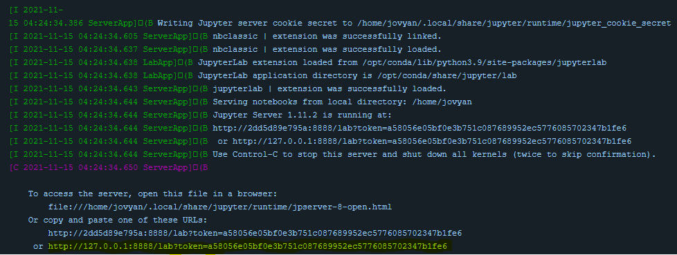
Figure 3.4 – Jupyter Docker logs
After opening up the notebook named chapter3.ipynb, you'll be greeted by the first cell of the notebook, which sets up the PySpark environment for you. The Docker image being used already includes the pyarrow module in the image, so it's already accessible for us to use. By clicking on the first cell and pressing the Shift + Enter keys, you'll start up the Spark master and executor, which will also download the necessary package for accessing AWS S3 from Spark. It should look similar to Figure 3.5:
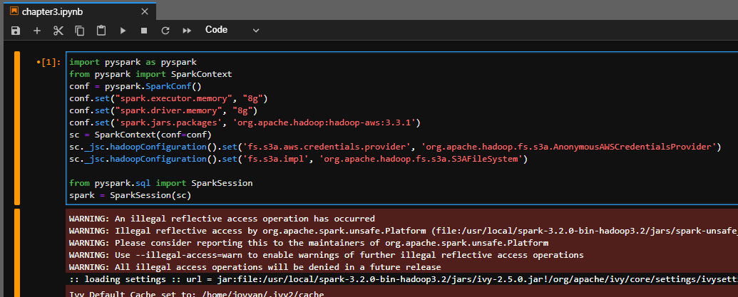
Figure 3.5 – Screenshot of provided Jupyter notebook
Now, you're all set to try running the examples I'm going to walk you through. You can see exactly how you'd be able to benefit from the Arrow integration in Spark. Let's begin!
SPARKing joy with Arrow and PySpark
So, looking at the files that are included, there are two of interest: sliced.csv and sliced.parquet. These are the aforementioned slices of the NYC Taxi dataset that we're going to use for these examples.
Setting Up the Data
The sliced.parquet file is included in the GitHub repository sample_data directory. The first cell of the Jupyter notebook for Chapter3 contains some quick code to write out the CSV file from the Parquet file. This way you don't have a large file to download.
The CSV file is around 511 MB, while the Parquet file is only 78 MB. Important to note is that they both contain the exact same data! That difference in file size is all down to the benefits of a binary, columnar storage format such as Parquet and the compression it uses. In addition to showing how to get our data into Spark from the CSV file, we're also going to see how much faster it is to get the same data usable from a Parquet file instead.
Step 1 – Making the data usable
The first thing I want you to do is to think back to the previous chapter and try to read that sliced.csv file into a pandas DataFrame Remember that Shift + Enter will run the code in the cell, or you can switch to just using a direct interactive console if you prefer it over the notebook. One cool thing you can use here is by prefacing a single line with %time before executing it, you'll get timing information printed out after execution. For multi-line cells, you just use an extra percentage sign, %%time. So, let's read that file into a DataFrame:
%%time
import pyarrow as pa
import pyarrow.csv
pdf = pa.csv.read_csv('../sample_data/sliced.csv').to_pandas()This is the output I get on my laptop. Your exact time might vary based on the specs of the machine you run the examples on:
CPU times: user 5.76 s, sys: 1.86, total: 7.63
Wall time: 1.86 s
Note
In case you are unfamiliar with the terms, wall time is the amount of time that elapsed if you used a stopwatch and timed the whole command. User time is the amount of CPU time utilized; on a machine with multiple cores, this can be much larger than the wall time. In this case, we know that by default, pyarrow is going to use multiple threads to read the CSV file, leading to a larger user time than wall time. Sys time is the time taken by the kernel to execute system-level operations such as context switching and resource allocation.
You may notice this as different from the output I used for timing in previous examples; the difference there is the usage of %timeit versus %time. Using %timeit will run the command several times in a loop and then give the average and standard deviation of the runtimes and tell you how many times it ran. Using %%timeit on the same code, I get the following output:
1.85 s ± 31.2 ms per loop (mean ± std. dev. of 7 runs, 1 loop each)
Either way, we see that it takes nearly 2 seconds on average (on my laptop) to read this CSV file into a pandas DataFrame using pyarrow. But remember, we need a Spark DataFrame for Spark to use it! The way to do that is with a very helpful method on the spark session object called createDataFrame. Unfortunately, on a 3.5 million row by 21 column pandas DataFrame this is actually a potentially very expensive operation. On my machine, it ends up taking over an hour! Wow! What about if we just read it directly using Spark's own functions? Run this in a cell of the Jupyter notebook:
%time df = spark.read.format('csv').load('../sample_data/sliced.csv',inferSchema='true',
header='true')
This is the output I get on my machine:
CPU times: user 9.98 ms, sys: 637 µs, total: 10.6 ms
Wall time: 4.26 s
Well, that's quite the difference there. That's the cost of translation that I mentioned earlier regarding the different DataFrame formats. However, recent releases of Spark have added support to utilize pyarrow support to supercharge these operations and reduce copies. You can enable this behavior by running the following:
spark.conf.set("spark.sql.execution.arrow.pyspark.enabled", "true")That's all. With this configuration set, we see a huge difference in how long it takes:
%time df = spark.createDataFrame(pa.csv.read_csv('../sample_data/sliced.csv').to_pandas())The output is as follows:
CPU times: user 6.2 s sys: 2.64 s, total 8.84 s
Wall time: 3.35 s
By enabling the usage of Arrow optimizations with Spark, we can benefit from Arrow's extremely fast reading of the CSV file and we are faster than natively reading it in Spark (at least with a single executor) but are still able to get a Spark DataFrame at the end. There's also one additional benefit of using the pyarrow library to perform our CSV reading, the default type inference.
There are two columns in our CSV file that consist of timestamps: tpep_pickup_datetime and tpep_dropoff_datetime. The fastest way to read in the file with Spark is to treat all the columns as strings or if you know the schema of the file beforehand. That way Spark will lazily load your file and only read it when you run a function that expects results. If you want to let the schema get figured out by reading the file, you can set the inferSchema option to true, as we did in the previous example. While Spark does provide mechanisms to specify custom parsing of the CSV, the default behavior doesn't recognize the timestamp columns as such, inferring them to just be a string typed column when using the native spark parsing:
df.printSchema()
The output is as follows:
root
|-- VendorID: integer (nullable = true)
|-- tpep_pickup_datetime: string (nullable = true)
|-- tpep_dropoff_datetime: string (nullable = true)
…
But, the pyarrow module has better default parsing and automatically recognizes those columns as timestamps, keeping them typed when converting to a pandas DataFrame. This means that the resulting Spark DataFrame maintains treating them as timestamps off the bat instead of having to separately cast them after reading the data in. This also applies to other types of parsing and type handling where the Arrow library is different, such as identifying certain columns as long whereas Spark reads them in as integer:
root
|-- VendorID: long
|-- tpep_pickup_datetime: timestamp (nullable = true)
|-- tpep_dropoff_datetime: timestamp (nullable = true)
Make sure to keep these differences in mind when using this, but don't forget about the customization options that exist for controlling what types get used, as seen in the previous chapter and the documentation.
While this is a fairly trivial example of converting a pandas DataFrame into a Spark DataFrame with the advent of so many libraries and modules that work directly with the pandas library, there are many cases where your pre-analysis operations for cleaning or manipulating the data will leave you with a pandas DataFrame at the end. This integration with Spark ensures superior performance for those cases where it isn't feasible to simply read the data directly into Spark natively due to your data pipeline's configuration.
Keep in Mind!
This is still an example of only using a single executor with my local machine. The benefit of Spark in general is the parallelization across multiple machines and cores, which I'm not using in the example here. You can still benefit from it using the Arrow library, but it's not as straightforward. The same is true for the Parquet version. If your dataset is large enough, you should use separate Spark tasks to create multiple smaller DataFrames and utilize the block_size and skip_rows_after_names read options for the CSV reader or read smaller row groups from the Parquet files.
Because of the optimizations and lazy loading, the speedup isn't as obvious with the Parquet file version just from reading it in. Regardless of whether you're using pyarrow directly or using Spark, it's going to read the Parquet file into your DataFrame in less than a second. But, if we use describe().show() to force Spark to read the entire file and perform some operations on it, we can see the benefits by using pyarrow to read the Parquet file over Spark's native parquet reader:
%%time
df = spark.read.format('parquet').load('../sample_data/sliced.parquet') # using pyspark native readerdf.describe().show()
We get the following output, though I've omitted the data itself to just show the resulting CPU and wall time that is reported:
…
CPU times: user 12.7 ms, sys: 247 µs, total: 12.9 ms
Wall time: 32.7 s
Looking at the timing information from using the Spark native reader, we can see how the work is done by the Spark driver and executors rather than the Python process. Despite the 32-second wall time, the CPU time reported is only a few milliseconds because all the work is done by the JVM process and Spark processes, and then just the results are sent back over from the JVM to the Python process. If we use pyarrow to read the file instead, we see the difference:
%%time
df = spark.createDataFrame(pq.read_table('../sample_data/sliced.parquet').to_pandas()) # using pyarrowdf.describe().show()
Once again, omitting the raw data, we get the following times as output:
…
CPU times: user 2.54 s, sys: 1.38 s, total: 3.92 s
Wall time: 12.3 s
Our timing shows a total of 3.92 seconds spent by the Python process as opposed to the 12.9 milliseconds from before. This is because the work to read the Parquet file is being done in Python by the pyarrow module, but the zero-copy benefits of the conversion and enabling Arrow in Spark make the data translation very fast. If we look at the Spark visualization of the execution plan for each side by side in Figure 3.6, it helps us understand what's going on:
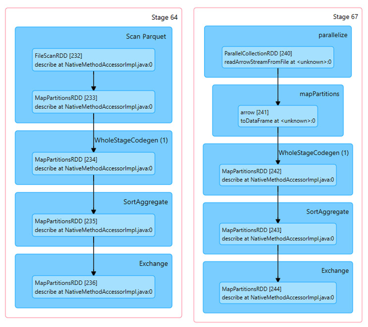
Figure 3.6 – Spark plans for native read versus Arrow -> pandas
Comparing the execution plans, the differences that we can see are the ParallelCollectionRDD and Arrow toDataFrame steps instead of FileScanRDD. It looks like Spark does a better job parallelizing the tasks when streaming arrow record batches than if Spark is doing the read directly. The pyarrow module reads the entire Parquet file into memory and then uses the Arrow inter-process communication (IPC) format to pass it to Spark in an easy to parallelize way. This becomes even more apparent if we look at the execution timelines for the two cases, as in Figure 3.7:
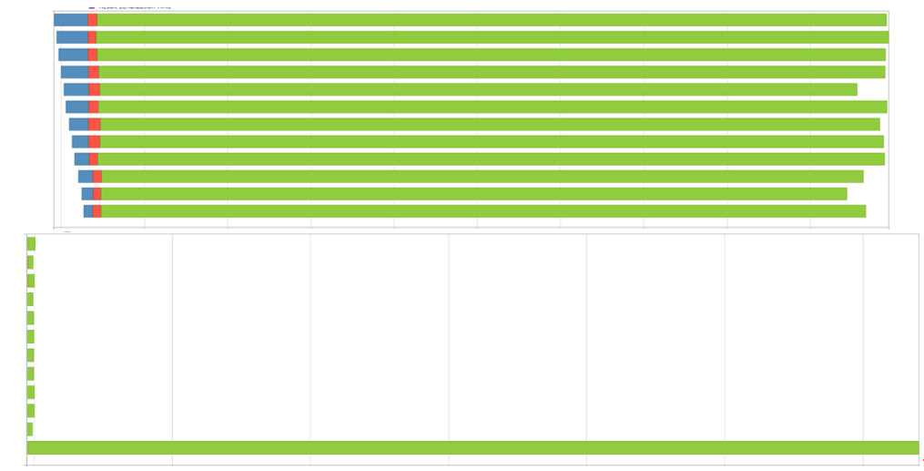
Figure 3.7 – Spark execution timelines for native and DataFrame Parquet
Can you guess which screenshot is from the run that used Arrow to read the file and pass the DataFrames? I'll give you a second… Yes, the top one. What you're looking at is how Spark chose to split the tasks up across different worker processes the driver used. The colors in the images represent how the time was spent by the executors. The blue sections are the scheduler delay and the red sections are the time deserializing the task. The green section is what we're most interested in, the time spent actually executing the task.
In both cases, Spark split up the work into 12 tasks, but in the case where it was streaming the Arrow record batches that were already read, instead of reading the file itself, the work got distributed much more evenly across all the workers, which each took a chunk of work. When Spark read the file itself, it only parallelized the read of the Parquet file to gather all the data into one executor that did all the computations resulting in the extra computation time it took.
For the purposes of the next steps, we only need a subset of the columns, which further improves our read performance:
- First we have the Spark native version:
%%timeit
df = spark.read.format('csv').load('../sample_data/sliced.csv',
inferSchema='true',
header='true').select('VendorID', 'tpep_pickup_datetime', 'passenger_count',
'tip_amount', 'fare_amount', 'total_amount')
5.28 s ± 216 ms per loop (mean ± std. dev. of 7 runs, 1 loop each)
- Then, using pyarrow and converting to a pandas DataFrame first:
% % timeit
df = spark.createDataFrame(pa.csv.read_csv('../sample_data/sliced.csv',
convert_options = pa.csv.ConvertOptions(
include_columns = ['VendorID', 'tpep_pickup_datetime',
'passenger_count', 'tip_amount',
'fare_amount', 'total_amount'
])
).to_pandas())
1.98 s± 104 ms per loop(mean± std.dev.of 7 runs, 1 loop each)
By taking advantage of the Arrow library's better read performance and the zero-copy conversion, we can demonstrate a significant performance improvement over using the native Spark loading functions.
Step 2 – Adding a new column
We're going to normalize our total_amount column by grouping rows based on the vendor ID and the month in which the trip occurred. Since we only have a full timestamp, we first need to add a column to our DataFrame that extracts the month from the timestamp.
For our DataFrame created by the Spark native reader that didn't automatically figure out the column as a timestamp type, we first need to cast that column to the right type before we can extract the month:
from pyspark.sql.functions import *
# import the functions we want to use like 'month',
# 'to_timestamp' and 'col'. Very useful.
df = df.withColumn('tpep_pickup_datetime', to_timestamp(col('tpep_pickup_datetime'), 'yyyy-MM-dd HH:mm:ss')) # the datetime format
With our properly typed datetime column in hand, we can add our new column, which extracts the month as a number so we can group by it easily:
df = df.withColumn('pickup_month', month(col('tpep_pickup_datetime')))Now, we can finally perform our normalization. Hold on to your hats, this is a doozy! We're going to use a user-defined function (UDF). You could do this with the native Spark intrinsic functions, but doing the normalization as a UDF is a stand-in for whatever complex logic you might have that is written in Python already. This allows you to avoid re-writing it or to benefit from the ease of writing Python without sacrificing performance. The reason why they exist is simply that there are a lot of computations and logic that are much more easily expressed using Python than with Spark's built-in functions, such as the following:
- Weighted mean
- Weighted correlation
- Exponential moving average
Step 3 – Creating our UDF to normalize a column
For this example, we're going to do a simple normalization of the total_amount column. The standard formula for normalization is as follows:

Note
Before I continue, I want to first acknowledge that I adapted this example from a fantastic webinar presentation given by Julien Le Dem and Li Jin that introduced this functionality. They go into significantly more detail, making the webinar a very worthwhile watch, so please give it a look when you have a chance. You can find it here: https://www.dremio.com/webinars/improving-python-spark-performance-interoperability-apache-arrow/.
The interesting thing to remember is that when you create a UDF in PySpark, it will execute your function in Python, not in the native Java/Scala that Spark runs in. As a result, UDFs are much slower to run than their built-in equivalents but are easier and quicker to write.
- Row-oriented functions – Operate on a single row at a time:
- lambda x: x + 1
- lambda date1, date2: (date1 – date2).years
- Grouped functions – Need more than one row to compute:
- Compute a weighted mean grouped by month
For the purposes of our example, and to show off the benefits of Apache Arrow, we're going to focus on the grouped UDF.
When building our user-defined monthly data normalization function, it's going to require a bunch of boilerplate code to pack and unpack multiple rows into a nested row that we can compute across. Because of this, performance is affected, as Spark first has to materialize the groups and then convert them to Python data structures so it can run the UDF, which is expensive. Let's take a crack at this; try working through the example here before looking at the notebook that has the solutions:
- First, to save ourselves some typing, let's import the PySpark SQL type functions:
from pyspark.sql.types import *
- Next, we need to create a struct column to represent our nested rows:
group_cols = ['VendorID', 'pickup_month']
non_group_cols = [col for col in df.columns if col not in
group_cols]
s = StructType([f for f in df.schema.fields if f.name in
non_group_cols])
cols = list([col(name) for name in non_group_cols])
df_norm = df.withColumn('values', struct(*cols))
- Now, we need to use our grouping definition to aggregate the values in the DataFrame:
df_norm = (df_norm
.groupBy(*group_cols)
.agg(collect_list(df_norm.values)
.alias('values')))
- See what I mean with all the boilerplate? Okay, next, we need to actually define our UDF to perform the normalization:
s2 = StructType(s.fields + [StructField('v', DoubleType())])
@udf(ArrayType(s2))
def normalize(values):
v1 = pd.Series([r.total_amount for r in values])
v1_norm = (v1 – v1.mean())/v1.std()
return [values[i] + (float(v1_norm[i]),)
for i in range(0, len(values))]
- We're almost there. We've got our normalization function, so we just have to apply it, explode the columns, and drop the extra columns we only needed for the calculation:
df_norm = (df_norm.withColumn('new_values',
normalize(df_norm.values))
.drop('values')
.withColumn('new_values',
explode(col('new_values'))))
for c in [f.name for f in s2.fields]:
df_norm = df_norm.withColumn(c,
col('new_values.{0}'.format(c)))
df_norm = df_norm.drop('new_values')
df_norm.show()
The highlighted line is what kicks off Spark to perform the work and start calculating everything. Before that point, it's just creating the plan until we want it to show us the results.
With everything in place, we can toss the %%time magic as the first line, and then run it so we can see how long it takes:
CPU times: user 74ms, sys: 53.5 ms, total: 127 ms
Wall time: 3min 9s
Okay. So that took a bit to run. Notice that the CPU timing shows that the Python process only spent about 127 milliseconds to construct the plan and send it to the JVM. The 3 minutes of runtime all took place within the JVM process and the Python processes Spark kicked off to run the UDF we created. For such a simple calculation, 3 minutes seems like a long time, even if it is for 3.5 million rows. Why did it take so long? Let's see the reasons in the following points:
- We had to pack and unpack the nested rows to get the data where we needed it.
- There was lots of serialization/deserialization to pass the data around. Spark, by default, is going to use the Python pickle protocol.
- The computation is still technically a scalar computation, so we're paying the costs of overhead for the Python interpreter and working with the row-by-row model instead of a column-oriented model.
Can we do better than this and also clean it up to remove a lot of the boilerplate? Of course we can, otherwise, I wouldn't have used this as an example!
Step 4 – Throwing out step 3 and using a vectorized UDF instead
First, I'm going to show the vectorized computation example, then I'll explain the differences in depth. So, let's take a look.
Are you ready? Here's the vectorized UDF and how to use it:
schema = StructType(df.schema.fields +
[StructField('v', DoubleType())])def vector_normalize(values):
v1 = values.total_amount
values['v'] = (v1 – v1.mean())/v1.std()
return values
group_columns = ['VendorID', 'pickup_month']
df_pandas_norm = df.groupby(*group_columns)
.applyInPandas(vector_normalize,
schema=schema)
df_pandas_norm.show()
That's it. That's everything. You should see the same output that you saw for Step 3, only much faster. How much faster? Well, shove the magic %%time keyword on that UDF, and let's find out together:
CPU times: user 22.1 ms, sys: 16.9 ms, total: 39 ms
Wall time: 3.57 s
That's 3.57 seconds instead of 3 minutes and 9 seconds. That's a huge 98.11% reduction in the time to calculate! So, how do we do it? Why does this run so much faster? The devil is in the details.
Step 5 – Understanding what's going on
To understand why vectorization of the calculation provides such a huge benefit, first, you have to understand how PySpark UDFs get calculated in the first place. Figure 3.8 is a simplified diagram of this execution:
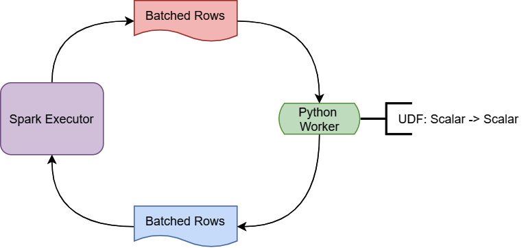
Figure 3.8 – PySpark UDF execution
During the execution of a UDF, the Spark executor running on Java/Scala is going to stream batches of rows to a Python worker. That worker is simply going to use a for loop to invoke the UDF on each row it gets and send back the results as another batch of rows. Given that the Spark executor is running in an entirely different programming language and runtime environment from the Python worker, you can guess that one of the big pieces of overhead is the serialization and deserialization of the data to send it back and forth between the environments. On top of that, since this is still a scalar computation, looping on a row-by-row basis isn't the most efficient way to perform the calculation. But, if we can take advantage of the vectorized, columnar computations that are implemented in pandas and eliminate the serialization/deserialization as seen in Figure 3.9, we end up with superior performance:
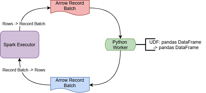
Figure 3.9 – Vectorized PySpark UDF
There are also other ways to leverage the vectorized computing for pandas within Spark:
- mapInPandas can be used instead of applyInPandas for applying a function through an iterator instead of a group-based operation, such as filtering rows by some criteria.
- When not grouping the data by some value, a simple pandas UDF can be used for performing vectorized element-wise operations, such as multiplying one column by another as a faster alternative to traditional Spark UDFs.
- Performing grouped aggregations, such as just calculating the mean/standard deviation of a given column, can be sped up using pandas_udf in conjunction with Windows functions and otherwise, instead of the traditional udf decorator.
Deeper information can be found in the Spark Python documentation for working with pandas and Arrow, but hopefully, the previous examples can get you started showing the power of utilizing the vectorized columnar calculations for your UDFs.
Step 6 – Profiting from our hard work
At the end of the day, the common development environment for data scientists of Jupyter and Apache Spark is yet another tool that is able to leverage Arrow for performance. As we can see, every step of the process, from loading the data files to performing computations on them, has the potential to benefit from the common memory format Arrow provides. After you've done your data normalization, cleanup, and any other modifications to the dataset that you want to do, what do we do next?
Raw data and numbers are all well and good, but to really get your point across, you want to provide charts and visual aids with your data. Well, there's a handy library called Perspective that utilizes Arrow built for visualizing data with charts and graphs and interactively manipulating those visuals. It's an open source interactive analytics and data visualization component that also includes a plugin for Jupyter allowing us to embed a widget to play with. The next section will show you how to take the data you've just prepared and feed it directly into Perspective to create useful charts and visuals directly from the Arrow formatted data.
Interactive charting powered by Arrow
Perspective was originally developed at J.P. Morgan and was open sourced through the Fintech Open Source Foundation (FINOS). The goal of this project was to make it easy to build analytics entirely in the browser that were user-configurable, or by using Python and/or Jupyter to create reports, dashboards, or any other application both with static data and streaming updates. It uses Apache Arrow as its underlying memory handler with a query engine built in C++ that is then compiled both for WebAssembly (for the browser/Node.js) or as a Python extension. While I highly encourage looking into it further, we're just going to cover using the PerspectiveWidget component for a Jupyter notebook to further analyze and play with the data we were using for the Spark examples, the NYC Taxi dataset.
Before we dive in, make sure that your Jupyter notebook is either still running, or you've spun it back up, as we're going to utilize it for this exercise. One of the cool, magic things Jupyter exposes is the ability to run commands as part of your notebook. In a cell of your notebook, you can place the following command to install the Python Perspective library:
!pip install perspective-python
Then, press the Shift + Enter keys to execute that and install it. Now, we can install the extension for the widget:
!jupyter labextension install @finos/perspective-jupyterlab
You're going to need to refresh your browser view of the Jupyter notebook after it finishes installing and rebuilding; you could also install this via the Jupyter UI. Also, make sure that you have the ipywidgets extension installed, which you can install with this command if you don't:
!jupyter labextension install @jupyter-widgets/jupyterlab-manager
Just like the Perspective widget extension, you can install this from the Jupyter UI if you prefer.
With our freshly refreshed instance of Jupyter running with the extensions, we're now ready to get a widget up to play with. Just follow along with these steps:
- First, we're going to import our data into an Arrow table in memory just like before. Try doing it yourself before reading further:
import pyarrow as pa
import pyarrow.csv
arrow_table = pa.csv.read_csv('../sample_data/sliced.csv')
- Next, we import the dependencies we're going to need for Perspective:
from perspective import Table, PerspectiveWidget
from datetime import date, datetime
import pandas as pd
- There are a few ways we could go from here. Perspective tables can be created from a pandas DataFrame or a dict object, but the most efficient by far is to just use Arrow directly. Perspective isn't able to take an Arrow table object directly, but it can read the Arrow IPC format if we just give the constructor the raw bytes:
sink = pa.BufferOutputStream() # create our buffer stream
with pa.ipc.new_stream(sink, arrow_table.schema) as writer:
writer.write_table(arrow_table) # write the table as IPC
buf = sink.getvalue() # get a buffer of the resulting bytes
Another alternative might be to have our dataset as a .arrow file written somewhere, which is just the Arrow IPC file format, as we've already covered.
- Finally, we can create our Perspective table, and to cut down on the render time, let's filter out some rows to bring it down to just under a million rows for us to play with:
table = Table(buf.to_pybytes())
view = table.view(filter=[
['tpep_pickup_datetime', '<', '2015-01-10']])
display(view.num_rows())
Running this gives us the output of the number of rows:
977730
- To create our widget from this view, we just call the to_arrow function on it to flatten it out to a new table for the widget to run over. In an actual production scenario, you might use a Python Tornado server to host the data remotely or to perform real-time updates of the data, but for now, a static dataset is fine:
widget = PerspectiveWidget(view.to_arrow())
widget
That's all that's necessary to get our initial widget drawn. Various arguments exist for the constructor so that you can control the initial state of the widget, such as the following:
- The initial view (Datagrid, Bar chart, Scatterplot, Heatmap, Treemap, Sunburst, and so on)
- The initial pivots of the rows and columns for grouping and splitting the dataset
- The initial sort order
- An initial subset of columns to display instead of showing all of them
- Further filters and custom columns derived from the existing columns
Figure 3.10 is a screenshot of this widget in action, where I've added some custom columns to split the pickup timestamp into the hour of the day and the day of the week:
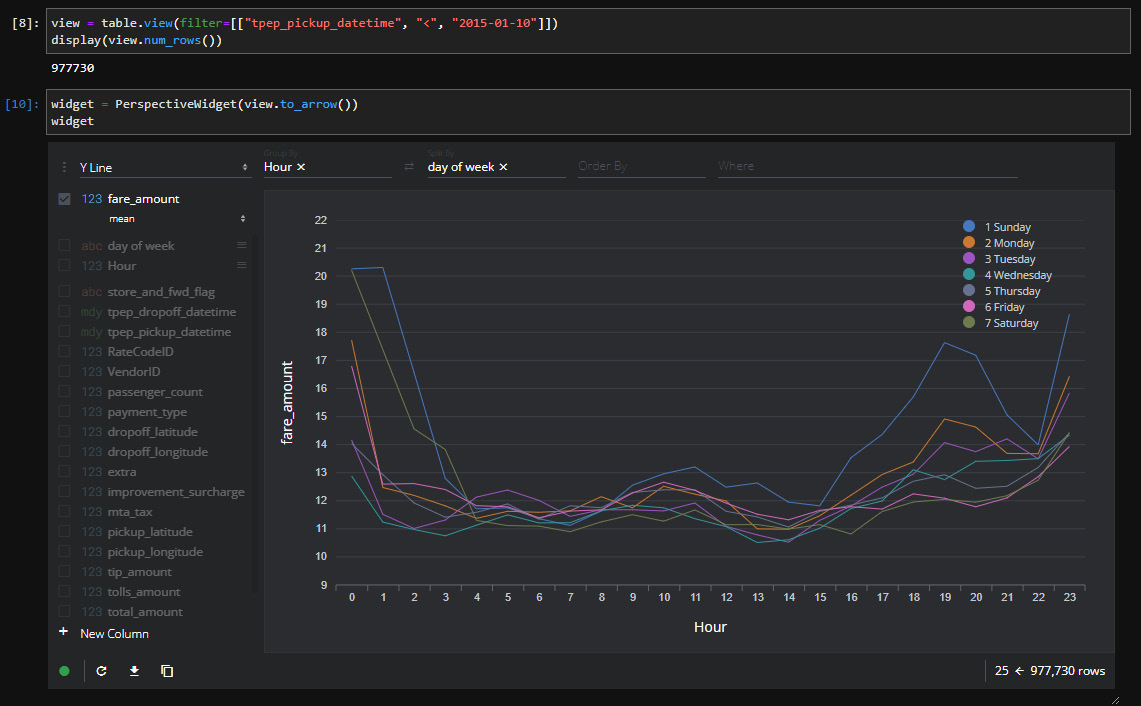
Figure 3.10 – Perspective widget inside of JupyterLab
Looking at Figure 3.10, you can see that I've grouped the input data by the fare amount field to create a chart showing the mean fare amount per hour for each day of the week. There are a lot of different options for how you want to display the data visually, enabling users to interactively manipulate what you're grouping by, splitting by, and so on. Another quick example is shown in Figure 3.11, which contains a heatmap for the average number of passengers per hour based on the days of the week. All I did was change the settings and wait a couple of seconds for the widget to update:
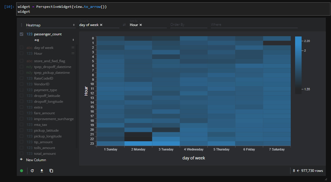
Figure 3.11 – Perspective widget heatmap
In this situation, the performance of this interactive charting widget is going to be directly connected to the power of your machine/given to your Docker machine running Jupyter. If you desire a bit more horsepower, you could use the Perspective documentation to create a server and build your own UI using the building blocks it provides. But this isn't a book about Perspective; I'm just using it as an example of what people have done and can do using Arrow.
While Perspective is an excellent example of adopting Arrow for an interactive data visualization solution, it's not the only attempt at this. A couple of other visualization solutions for Arrow formatted data that I've come across are as follows:
- Falcon: A visualization tool for linked interactions across multiple aggregate visualizations (github.com/vega/falcon)
- Vega: An ecosystem of tools for interactive web-based visualizations (github.com/vega)
- Graphistry: A company providing utilities and specialized hardware to use GPUs to accelerate visualization of large datasets using Arrow and remote rendering (graphistry.com/data-science)
After covering all these analytics use cases, there's one use case that we're leaving out a bit: searching. While Arrow can supercharge your analytics engines, improve your data transfer, and make it seamless to share data between programming languages, very few tools are able to beat the power of Elasticsearch when it comes to just performing searches and simple aggregations. Recently, I worked on an application whose analytics were powered on analytics engines using Apache Arrow, but we found that after pre-calculating all the data, Elasticsearch was the best method to return pages of data to the UI.
Stretching workflows onto Elasticsearch
If what you need is primarily searching and filtering large amounts of data rather than heavy analytical computations, chances are you've probably looked into Elasticsearch. Even if you do need heavy computations, you might be able to pre-calculate large amounts of data and store it in Elasticsearch to fetch later to speed up your queries. However, there's a slight issue: Elasticsearch's API is entirely built in JSON, and Arrow is a binary format. We also don't want to sacrifice our fast data transportation using Arrow's IPC format if we can avoid it!
I recently worked on a project where the solution we came up with was to have a unified service interface that used Arrow, but heuristically determine when a request would be better serviced by an Elasticsearch query and simply convert the data from the JSON returned by Elasticsearch to Arrow. If this seems overly complicated, here's what this solution achieved for us:
- A unified interface for consumers:
- Regardless of the underlying data source, our consumers got data using the Arrow IPC format with a proper schema.
- Separation of concerns:
- If something better comes along for this particular use case, we can easily replace Elasticsearch with it and consumers won't have to care or be affected.
- An optimized interface for bulk fetches that use Arrow the whole way through:
- Elasticsearch works best if the result data from a given fetch is relatively small rather than trying to fetch your entire dataset at once. That small result set is quick to convert to Arrow from JSON. Big bulk fetches that would be very expensive to convert instead come from a bulk interface that just returns Arrow natively.
Since the data is stored using Parquet files or accessed by a native Arrow format interface, the first thing we had to do was work out how to get the data indexed by Elasticsearch in the first place. Thankfully, this turned out to not be difficult, as several Arrow libraries have easy conversions to JSON that work very well for mapping to Elasticsearch documents. Once all of the data was indexed, the service we built would determine whether to query Elasticsearch or a different source based on the request, and if Elasticsearch was queried, the JSON response would get converted back to Arrow before it was returned. Visually, the architecture looked like Figure 3.12:
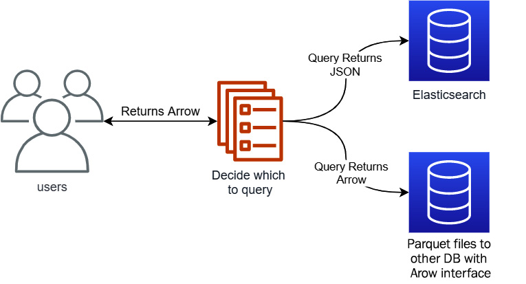
Figure 3.12 – Service architecture including Elasticsearch
Let's take a look at the interaction with Elasticsearch and how the conversion to and from JSON works in this case. We'll launch an instance of Elasticsearch locally using Docker with the following command:
$ docker run -–rm -it -p 9200:9200 -p 9300:9300 -e "discovery.type=single-node" docker.elastic.co/elasticsearch/elasticsearch:7.15.2
After it starts up and is running, you can visit http://localhost:9200 in your browser to confirm it is up and running. You should see something similar to this in your browser:
{"name": "21c57c172ae9",
"cluster_name": "docker-cluster",
"cluster_uuid": "ZAm29KdFS6e2osGXY44vvQ",
"version": {"number": "7.15.2",
"build_flavor": "default",
"build_type": "docker",
"build_hash": "93d5a7f6192e8a1a12e154a2b81bf6fa7309da0c",
"build_date": "2021-11-04T14:04:42.515624022Z",
"build_snapshot": false,
"lucene_version": "8.9.0",
"minimum_wire_compatibility_version": "6.8.0",
"minimum_index_compatibility_version": "6.0.0-beta1"
},
"tagline": "You Know, for Search"
}
With an Elasticsearch instance now running locally on your laptop, we can start filling it with data for us to query. Keep in mind that Elasticsearch is not intended to be the source of truth for your data; it's an optimization for querying with particular workflows. Referencing the architecture diagram from Figure 3.12, we created automated jobs that performed updates of the data in Elasticsearch when the underlying data in Parquet files changed or updated.
Indexing the data
Using the Parquet files or database that returns native Arrow as the source of truth, Elasticsearch can be easily populated after converting the Arrow data to JSON, as long as you take care when handling the data types. When creating an index in Elasticsearch, you have two choices for handling the data types: dynamic mapping and explicit mapping. Because of the flexible nature of JSON, when converting from Arrow, it makes more sense to use an explicit mapping since you already know the data types via the Arrow schema. You can see the data types that Elasticsearch supports in the documentation available online (https://www.elastic.co/guide/en/elasticsearch/reference/current/mapping-types.html). Most of the type mapping can be handled with some simple mappings, but for other types such as dates, times, and strings, you'll want to include extra information to handle the mapping. I'm going to use Go for these examples, but conceptually, this would work with the Arrow library in any language:
- First, let's create a struct to make it easy to marshal the mapping to JSON:
type property struct {
Type string `json:"type"`
Format string `json:"format,omitempty"`
Fields interface{} `json:"fields,omitempty"`
}
If you're unfamiliar with Go, the `json:"format,omitempty"` tags in the struct definition define how an instance of this struct would get marshaled to JSON. The omitempty tag tells the marshaller to leave out this field if it is empty, which is defined differently based on the type. For a string, empty is just when the length is 0. For interface{}, empty is when the value is nil.
- For this example, we're going to create a static keyword field definition with defaults to use for string values, but this could be replaced by more specific options if desired:
var keywordField = &struct{
Keyword interface{} `json:"keyword"`
}{struct {
Type string `json:"type"`
IgnoreAbove int `json:"ignore_above"`
}{"keyword", 256}}
- Now, let's create our simple mapping for the primitive values:
import (
…
"github.com/apache/arrow/go/v7/arrow"
…
)
var primitiveMapping = map[arrow.Type]string{
arrow.BOOL: "boolean",
arrow.INT8: "byte",
arrow.UINT8: "short", // no unsigned byte type
arrow.INT16: "short",
arrow.UINT16: "integer", // no unsigned short
arrow.INT32: "integer",
/* the rest of the arrow types */
}
- Finally, let's construct a function that converts an Arrow schema to mapping for JSON conversion. For this example, I'm not going to handle nested types such as Union, List, Struct, or Map columns, but they could be easily handled with Elasticsearch's type system, which allows array and object types:
func createMapping(sc *arrow.Schema) map[string]property {
mappings := make(map[string]property)
for _, f := range sc.Fields() {
var (
p property
ok bool
)
if p.Type, ok = primitiveMapping[f.Type.ID()]; !ok {
switch f.Type.ID() {
case arrow.DATE32, arrow.DATE64:
p.Type = "date"
p.Format = "yyyy-MM-dd"
case arrow.TIME32, arrow.TIME64:
p.Type = "date"
p.Format = "time||time_no_millis"
case arrow.TIMESTAMP:
p.Type = "date"
p.Format = "yyyy-MM-dd HH:mm:ss||yyyy-MM-dd HH:mm:ss.SSSSSSSSS"
case arrow.STRING:
p.Type = "text" // or keyword
p.Fields = keywordField
}
}
mappings[f.Name] = p
}
return mappings
}
Walking through the code snippet, the first highlighted section checks whether the type of the field is in our primitive mapping. If it isn't, then we have to handle the type separately. The next several highlighted lines specify the expected string format that the JSON conversion will output the date, time, or timestamp to so that Elasticsearch knows what to expect for ingesting documents. In the case of a string, we can use either the text or keyword type and use the keyword field definition we made to tell Elasticsearch to index the value accordingly.
- We've got our helper functions, so now we need some data. Let's read from the Parquet file in the sample data named sliced.parquet. Many of the official Parquet libraries provide an easy reader that reads data directly into Arrow record batches; the Go library does this through a module named pqarrow:
import (
…
"github.com/apache/arrow/go/v7/arrow/memory"
"github.com/apache/arrow/go/v7/parquet/file"
"github.com/apache/arrow/go/v7/parquet/pqarrow"
…
)
func main() {
// the second argument is a bool value for memory mapping
// the file if desired.
parq, err := file.OpenParquetFile("../../sample_data/sliced.parquet", false)
if err != nil {
// handle the error
}
defer parq.Close()
props := pqarrow.ArrowReadProperties{BatchSize: 50000}
rdr, err := pqarrow.NewFileReader(parq, props,
memory.DefaultAllocator)
if err != nil {
// handle error
}
…
}
The pqarrow module provides helper functions that can read an entire file into memory as an Arrow table, but we want to limit the amount of memory we're using. So, rather than pulling the entire file into memory at one time, we create a Parquet file reader and wrap that with a pqarrow reader. We create a properties object and define the batch size to use, which is the number of rows that will be read from a column per read. Higher batch sizes can speed up the indexing but will require more memory.
- We're going to stream our records out of the file and to Elasticsearch, which means we're going to utilize a goroutine to concurrently read record batches and use the bulk index API of Elasticsearch. In order to ensure graceful failures, we're going to need a context and a cancel function. We can then use that context to create a record reader as per the highlighted lines as follows:
import (
"context"
…
)
func main() {
…
ctx, cancel := context.WithCancel( context.Background())
defer cancel()
// leave these empty since we're not filtering out any
// columns or row groups. But if you wanted to do so,
// this is how you'd optimize the read
var cols, rowgroups []int
rr, err := rdr.GetRecordReader(ctx, cols, rowgroups)
if err != nil {
// handle the error
}
…
}
- Huzzah! We can create our index in Elasticsearch now. For ease of use, the default client expects an environment variable to be set named ELASTICSEARCH_URL, which is the address of the Elasticsearch instance. If you're following along and used Docker to launch your instance, you can set the environment variable to the http://localhost:9200 value. First, let's add the necessary imports; your editor might be smart enough to do this automatically:
import (
"net/http"
…
"github.com/elastic/go-elasticsearch/v7"
"github.com/elastic/go-elasticsearch/v7/esutil"
…
)
Now, we add the creation of an Elasticsearch client to the main function:
…
es, err := elasticsearch.NewDefaultClient()
if err != nil {
// handle the error
}
…
Finally, we create our Elasticsearch index mappings from the schema of our RecordReader and create the index itself:
…
var mapping struct {
Mappings struct {
Properties map[string]property `json:"properties"`
} `json:"mappings"`
}
mapping.Mappings.Properties = createMapping(rr.Schema())
response, err := es.Indices.Create("indexname",
es.Indices.Create.WithBody(
esutil.NewJSONReader(mapping)))
if err != nil {
// handle error
}
if response.StatusCode != http.StatusOK {
// handle failure response and return/exit
}
// Index created!
…
Creating the index is straightforward as per the highlighted lines. We get the Arrow schema from the record reader and create an Elasticsearch client, then use our function to construct the mappings. The official Elasticsearch library provides a very useful utility package called esutil, which contains helpers such as the NewJSONReader function we call to convert the mapping struct to a JSON object and create io.Reader to send the request. If all goes well, the response should have the HTTP response code of 200, represented by the http.StatusOK constant.
- We're almost done! We've got our index created and we've got our record reader to pull batches of rows from the file. We just need to use the bulk indexer API to stream all of this into our instance. I know this is my longest code step list so far but stay with me now! This is the cool part. First, the extra imports we're going to need to finish this up are as follows:
import (
…
"bufio"
"io"
"strings"
"fmt"
…
"github.com/apache/arrow/go/v7/arrow/array"
)
- Then, we create our bulk indexer. There are a lot of options that exist on the indexer object to control the amount of parallelism it can use, how often to flush the data, and so on. We're just going to use the defaults for those options for now, but feel free to play with them:
…
indexer, err := esutil.NewBulkIndexer(esutil.BulkIndexerConfig{
Client: es, Index: "indexname",
OnError: func(_ context.Context, err error) {
fmt.Println(err)
},
})
if err != nil {
// handle error
}
- Let's start actually reading from the file into a pipe that we'll read lines from. Using array.RecordToJSON will convert the records to JSON with each row as a single-line JSON object, just as we saw in the previous chapter. We use the go func syntax to start a goroutine running concurrently with our indexer:
pr, pw := io.Pipe() // to pass the data
go func() {
for rr.Next() {
if err := array.RecordToJSON(rr.Record(), pw); err != nil {
cancel()
pw.CloseWithError(err)
return
}
}
pw.Close()
}()
- We can use bufio.Scanner to grab the JSON data line by line to send to Elasticsearch's bulk index API. Just initialize it to read from the read side of the pipe we created and we're off to the races! The highlighted lines are how we add the items to the bulk indexer, and the Scan method will return false when we hit the end of the data:
scanner := bufio.NewScanner(pr)
for scanner.Scan() {
err = indexer.Add(ctx, esutil.BulkIndexerItem{
Action: "index",
Body: strings.NewReader(scanner.Text()),
OnFailure: func(_ context.Context,
item esutil.BulkIndexerItem,
resp esutil.BulkIndexerResponseItem,
err error) {
fmt.Printf("Failure! %s, %+v %+v ", err, item, resp)
},
})
if err != nil {
// handle the error
}
}
if err = indexer.Close(ctx); err != nil {
// handle error
}
…
Okay, so that was a bit more complicated than I may have made it seem. The full code can be found in the GitHub repository for the book and I encourage you to try it out and play with the different settings and tweaks to control the performance, memory usage, and so on. Since you've seen the code to convert Arrow record batches to JSON for indexing into Elasticsearch, you should be able to build the reverse yourself! Write something that can take the response from an Elasticsearch query, which would be JSON objects, and reconstruct the Arrow record batches from it. Because of the format of Elasticsearch responses, it's not quite as simple as just directly using the JSON reader in the Arrow library. After you attempt this, you can take a look at the GitHub repository's Chapter3 directory for the solution.
Building the full service end to end is a bit outside the scope of this chapter, but I highly recommend taking a stab at it, as it makes a great exercise in most of the things we've covered so far. It's also pretty fun and a cool thing to see when it works, as it's extremely performant, if you like that sort of thing.
Summary
With Jupyter, Spark, and ODBC as some of the most ubiquitous utilities in data science, it only makes sense to cover Arrow from the perspective of its integration with these tools. Many of you will likely not use Arrow directly in these cases, but rather benefit from the work being done by others utilizing Arrow. But, if you're a library or utility builder, or just want to tinker a bit to see whether you can improve the performance of some different tasks, this chapter should have given you a lot of information to chew on and hopefully a bunch of ideas to try out, such as converting Arrow on the fly to populate an Elasticsearch index but maintain a consistent interface.
I don't want to give you all the answers, mostly because I don't have them. There's a wealth of people all over experimenting with Arrow in a large number of different use cases, some of which we'll cover in other chapters. Hopefully, this chapter, and the chapters to come after it, set you up with all the building blocks you need to create awesome things, either by leveraging Arrow to facilitate a new library or utility or by utilizing Arrow and those tools to analyze your data in increasingly faster ways.
The next chapter is Chapter 4, Format and Memory Handling. We're going to take a closer look at the various ways data is passed around and stored and discuss the relationships and use cases they are all trying to address. The goal is to see where Arrow and its IPC format can fit in the existing data ecosystem with the multitude of trade-offs, and pros and cons that exist for how something is used or implemented.
Onwards!